
Dragon Taming: Engineering Candlestick Factors for Monthly Backtests
In the previous installment, we reproduced the factor construction from the research report, specifically the upper shadow factor, the Williams lower shadow factor, and the combined UBL factor. In this issue, we will put these factors to the test.
While factor testing is an indispensable part of factor mining, it should be a routine task—we shouldn’t reinvent the wheel every time. However, when we attempted to use Alphalens for factor testing, an embarrassing situation arose.
Alphalens, Please Step Up
Alphalens is an open-source library built on pandas that provides a suite of functions for analyzing and evaluating factors. It has long been the go-to choice for factor testing.
So, let’s start by testing the upper shadow standard deviation factor.
def calculate_shadow_ratio(bars):
"""计算上下影线因子(归一化)
按研报要求,标准化蜡烛上影线为当日上影线/过去 5 日上影线均值。标准化蜡烛下影线同。
"""
high = bars['high']
low = bars['low']
open_price = bars['open']
close = bars['close']
# 为避免除零错误,这里我们使用了一个技巧,即通过 mask 来排除可能除零的计算
# 无法计算时,设置为 0,表明无信号
up_shadow_ratio = pd.Series(0, index=bars.index)
down_shadow_ratio = pd.Series(0, index=bars.index)
up_shadow = high - np.maximum(open_price, close)
rolling_up_shadow = up_shadow.rolling(5).mean()
mask = rolling_up_shadow > 1e-8
up_shadow_ratio[mask] = up_shadow[mask] / rolling_up_shadow[mask]
down_shadow = np.minimum(open_price, close) - low
rolling_down_shadow = down_shadow.rolling(5).mean()
mask = rolling_down_shadow > 1e-8
down_shadow_ratio[mask] = down_shadow[mask] / rolling_down_shadow[mask]
return up_shadow_ratio, down_shadow_ratio
def calc_monthly(daily_factor, aggfunc, win=20):
dates = daily_factor.index.get_level_values('date').unique().sort_values()
month_ends = dates.to_frame(name = "date").resample('BME').last().values
dfs = []
for date in month_ends:
date_ts = pd.Timestamp(date.item())
iend = dates.get_loc(date_ts)
istart = max(0, iend - win + 1)
start_ = pd.Timestamp(dates[istart])
end_ = date_ts
window_data = daily_factor.loc[start_: end_]
df = (window_data.groupby(level="asset")
.agg(aggfunc)
.to_frame("factor")
)
df["date"] = date_ts
dfs.append(df)
df = pd.concat(dfs)
return df.set_index(["date", df.index]).sort_index()
def calc_candle_up_std_factor(barss, win = 20):
up_shadow = barss.groupby("asset", group_keys=False).apply(lambda x: calculate_shadow_ratio(x)[0]).sort_index()
return calc_monthly(up_shadow, "std", win)These are the codes introduced in the previous issue. Now, let’s call Alphalens to run the test:
attention
```python from alphalens.performance import factor_alpha_beta start = datetime.date(2009,1,1 ) end = datetime.date(2020,4,30) barss = load_bars(start, end, 50)up_std_factor = calc_candle_up_std_factor(barss, 20)
prices = barss["price"].unstack(level = 1)
merged = get_clean_factor_and_forward_returns(up_std_factor, prices, quantiles=5)
alpha = factor_alpha_beta(merged)
alpha</div>
<!--PAID CONTENT END-->
<!-- BEGIN IPYNB STRIPOUT -->
```python
from alphalens.performance import factor_alpha_beta
start = datetime.date(2009,1,1 )
end = datetime.date(2020,4,30)
barss = load_bars(start, end, 50)
up_std_factor = calc_candle_up_std_factor(barss, 20)
prices = barss["price"].unstack(level = 1)
merged = get_clean_factor_and_forward_returns(up_std_factor, prices, quantiles=5)
alpha = factor_alpha_beta(merged)
alphaAs expected, an unexpected error occurred. Alphalens threw an exception:
warning
Don’t panic! This code is destined to fail. ```python File ~/miniforge3/envs/zillionare/lib/python3.12/site-packages/pandas/core/arrays/datetimelike.py:2162, in TimelikeOps._validate_frequency(cls, index, freq, **kwargs) 2156 raise err -> 2162 raise ValueError( 2163 f"Inferred frequency {inferred} from passed values " 2164 f"does not conform to passed frequency {freq.freqstr}" 2165 ) from errValueError: Inferred frequency None from passed values does not conform to passed frequency C</div>
The data returned by the `calc_candle_up_std_factor` function only contains dates at the end of each month. Alphalens cannot infer a trading calendar from this, hence the exception.
<div class="admonition admonition-tip"><p class="admonition-title">tip</p>
When performing factor return analysis, Alphalens first calculates forward returns. Forward returns are specified by the user via the `periods` parameter, defaulting to [1, 5, 10]. The unit for `periods` defaults to "Day," so it expects a date-continuous index. Since the data we passed only contained end-of-month dates, we received this exception.
</div>
Fundamentally, Alphalens cannot handle strategies with monthly rebalancing. A workaround recommended by Alphalens is to calculate the factor daily and specify the `periods` parameter as [21, 105, 210], thereby simulating forward returns calculated over 1, 5, and 10 months. However, this recommended workaround is not necessarily viable, as not every month has exactly 21 trading days.
## Introducing a Newcomer
Given that monthly factor testing is very common in research reports, we decided to develop a simple backtest library specifically for monthly factors. It will implement the following functionality: for each asset with data at the end of the month, we will buy at the opening price on the first day of the next month and sell at the closing price at the end of that month, calculating the return.
<div class="admonition admonition-tip"><p class="admonition-title">tip</p>
Another common rapid testing framework is vectorbt. Theoretically, it can implement the logic of buying at the beginning of the month and selling at the end, but this relies on individual implementation.
</div>
<!--PAID CONTENT START-->
The code is somewhat long, but the core logic lies in the following two functions:
```python
def _monthly_factor_backtest(
factor_data: "pd.Series[float]",
bars: pd.DataFrame,
quantiles: Optional[int] = 5,
bins: Optional[Union[int, List[float]]] = None,
factor_lag: int = 1,
weighting_method: str = "equal_weight",
) -> Tuple[
pd.DataFrame, "pd.Series[float]", "pd.Series[float]", "pd.Series[float]"
]:
"""
Monthly Factor Backtesting Framework
策略逻辑:
1. 基于上月末因子值对股票分组
2. 在下月初买入,下月末卖出
3. 计算各组合的月度收益率
如果因子值或者价格数据在交易日期(月初或者月末)缺少数据,该资产将被从组合中排除。这有可能导致回测数据不足。因此,推荐做法是您确保传入的因子数据和价格数据,都包含所有交易日期的数据。
Returns:
tuple: (策略分组月度收益 DataFrame, 基准月度收益 Series, long-only 收益 Series, 多空组合收益 Series, IC 序列 Series)
策略收益以月份为索引,分组为列
基准收益为所有股票等权重收益
纯多和多空组合收益根据 weighting_method 计算
IC 序列为每月因子值与收益率的相关系数
"""
# 重置索引便于操作
factor_df = factor_data.to_frame(name="factor").reset_index()
factor_col = "factor"
bars_df = bars.reset_index()
# 转换日期列为 datetime 类型
factor_df["date"] = pd.to_datetime(factor_df["date"])
bars_df["date"] = pd.to_datetime(bars_df["date"])
# 构建交易日历
trading_calendar = _build_trading_calendar(bars_df)
# 为因子数据添加年月信息
factor_df["year_month"] = factor_df["date"].dt.to_period("M")
# 存储月度收益
monthly_returns = []
benchmark_returns = []
long_only_returns = []
long_short_returns = []
ic_values = []
# 遍历交易日历,执行回测
for i in range(factor_lag, len(trading_calendar)):
current_trading_month = trading_calendar.iloc[i]
factor_month = trading_calendar.iloc[i - factor_lag]
# 处理单个月的回测逻辑
result = _process_single_month(
current_trading_month=current_trading_month,
factor_month=factor_month,
factor_df=factor_df,
bars_df=bars_df,
factor_col=factor_col,
quantiles=quantiles,
bins=bins,
weighting_method=weighting_method,
)
if result is not None:
(
group_returns,
benchmark_return,
long_only_return,
long_short_return,
ic_value,
) = result
monthly_returns.append(group_returns)
benchmark_returns.append(benchmark_return)
long_only_returns.append(long_only_return)
long_short_returns.append(long_short_return)
ic_values.append(ic_value)
# 合并所有月份的收益
if not monthly_returns:
return pd.DataFrame(), pd.Series(), pd.Series(), pd.Series(), pd.Series()
# 策略收益
quantile_returns = pd.concat(monthly_returns, axis=1).T
quantile_returns.index = cast(
pd.PeriodIndex, quantile_returns.index
).to_timestamp(how="end", freq="D")
# 重命名列
if quantiles is not None:
quantile_returns.columns = [f"Q{i}" for i in quantile_returns.columns]
else:
quantile_returns.columns = [f"Bin{i}" for i in quantile_returns.columns]
# 基准收益
benchmark_series = pd.Series(
benchmark_returns, index=quantile_returns.index, name="Benchmark"
)
# long-only 收益
long_only_series = pd.Series(
long_only_returns, index=quantile_returns.index, name="Long_Only"
)
# 多空组合收益
long_short_series = pd.Series(
long_short_returns, index=quantile_returns.index, name="Long_Short"
)
# IC 序列
ic_series = pd.Series(ic_values, index=quantile_returns.index, name="IC")
return (
quantile_returns,
benchmark_series,
long_only_series,
long_short_series,
ic_series,
)The single-month backtest function _process_single_month is defined as:
def _process_single_month(
self,
current_trading_month: "pd.Series[Any]",
factor_month: "pd.Series[Any]",
factor_df: pd.DataFrame,
bars_df: pd.DataFrame,
factor_col: str,
quantiles: Optional[int] = None,
bins: Optional[Union[int, List[float]]] = None,
weighting_method: str = "equal_weight",
) -> Optional[Tuple["pd.Series[float]", float, float, float, float]]:
"""
处理单个月的回测逻辑
"""
# 获取因子计算时点的数据(通常是月末)
factor_date = factor_month["month_end"]
factor_month_data = factor_df[(factor_df["date"] == factor_date)].copy()
if len(factor_month_data) == 0:
return None
# 买入价格(当月月初开盘价)
buy_date = current_trading_month["month_start"]
buy_prices = bars_df[bars_df["date"] == buy_date][["asset", "open"]].copy()
buy_prices.columns = ["asset", "price_buy"]
# 卖出价格(当月月末收盘价)
sell_date = current_trading_month["month_end"]
sell_prices = bars_df[bars_df["date"] == sell_date][["asset", "close"]].copy()
sell_prices.columns = ["asset", "price_sell"]
if len(buy_prices) == 0 or len(sell_prices) == 0:
return None
# 合并数据
month_data = factor_month_data.merge(buy_prices, on="asset", how="inner")
month_data = month_data.merge(sell_prices, on="asset", how="inner")
# 移除缺失数据的股票
month_data = month_data.dropna(subset=[factor_col, "price_buy", "price_sell"])
if len(month_data) == 0:
return None
# 因子分组
try:
if quantiles is not None:
month_data["group"] = (
pd.qcut(
month_data[factor_col],
q=quantiles,
labels=False,
duplicates="drop",
)
+ 1
)
else:
assert bins is not None, "bins 不能为 None"
month_data["group"] = (
pd.cut(
month_data[factor_col],
bins=bins,
labels=False,
include_lowest=True,
)
+ 1
)
except ValueError:
# 如果因子值相同导致无法分组,跳过该月
return None
# 计算个股收益率
month_data["return"] = month_data["price_sell"] / month_data["price_buy"] - 1
# 计算各组等权重收益率(保持原有逻辑)
group_returns = month_data.groupby("group")["return"].mean()
# 计算基准收益率(所有股票等权重)
benchmark_return = month_data["return"].mean()
# 计算 long-only 和多空组合收益率
long_only_return, long_short_return = self._calculate_portfolio_returns(
month_data, group_returns, factor_col, weighting_method
)
# 计算 IC 值(因子值与收益率的相关系数)
ic_value = month_data[factor_col].corr(month_data["return"])
if pd.isna(ic_value):
ic_value = 0.0
# 添加月份信息
group_returns.name = current_trading_month["year_month"]
return (
group_returns,
benchmark_return,
long_only_return,
long_short_return,
ic_value,
)The most critical part involves resampling the price data to generate a monthly calendar (with start-of-month and end-of-month dates). We can then iterate through the factors. For each factor value at the end of month T0, we find the corresponding start of the next month, buy at the opening price, and sell at the closing price at the end of that month. The resulting return is the monthly return for the T0 factor.
Finally, we return the group monthly returns, benchmark monthly returns, long-short hedge returns, single-month returns, and IC.
Using moonshot is straightforward.
First, let’s generate some data to demonstrate.
def key_frames(bars, dates):
df = dates.to_frame(name = "date")
month_starts = df.resample('MS')['date'].first()
month_ends = df.resample('BME')['date'].last()
key_frames = bars[
(bars.index.get_level_values(0).isin(month_ends) |
bars.index.get_level_values(0).isin(month_starts))
]
return key_frames
factor_data = [
(pd.Timestamp('2023-01-31'), "A", 1.0),
(pd.Timestamp('2023-01-31'), "B", 2.0)
]
factor_df = pd.DataFrame(factor_data,
columns=["date", "asset", "factor"]).set_index(["date", "asset"])
dates = pd.date_range('2023-01-01', '2023-02-28', freq='D')
prices = [("A", 100, 110), ("B", 100, 105)] * len(dates)
bars = pd.DataFrame(prices, columns=["asset", "open", "close"],
index=np.repeat(dates, 2))
bars = bars.set_index([bars.index, 'asset'])
bars.index.names = ["date", "asset"]
display(key_frames(bars, dates).unstack())
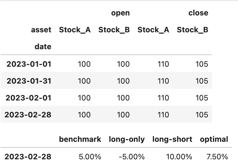
print("Stock_A (因子=1.0): 收益率 = (110-100)/100 = 10%")
print("Stock_B (因子=2.0): 收益率 = (105-100)/100 = 5%")
print("Q1组 (因子较小): Stock_A, 收益率 = 10%")
print("Q2组 (因子较大): Stock_B, 收益率 = 5%")
print("benchmark = (10% + 5%) / 2 = 7.5%")
expected = pd.DataFrame([[0.075, 0.05, -0.05, 0.1]],
columns=["benchmark", "long-only", "long-short", "optimal"], index=["2023-02-28"])
expected.style.background_gradient(cmap='RdYlGn')
expected.style.format("{:.2%}")Here is the data and the expected values:
Backtesting and result visualization require just three lines of code:
from moonshot import Moonshot
moonshot = Moonshot()
# 执行回测(使用2个分位数)
moonshot.backtest(factor_df, bars, quantiles=2)
actual = pd.DataFrame([moonshot.benchmark_returns,
moonshot.long_only_returns,
moonshot.long_short_returns,
moonshot.optimal_returns]).T
actual.columns = ["benchmark", "long-only", "long-short", "optimal"]
actual.style.format("{:.2%}")As expected, the results align perfectly with our expectations.
Can the Research Report Conclusions Be Reproduced?
Now that we understand how to use the backtesting tool, let’s answer the most critical question: Can the factors proposed in the research report be reproduced? We will use moonshot for factor testing.
Candlestick Upper Shadow Standard Deviation Factor
Let’s first look at the candlestick upper shadow standard deviation factor:
start = datetime.date(2009, 1, 1)
end = datetime.date(2020, 4, 30)
barss = load_bars(start, end, 50)
factor = calc_candle_up_std_factor(barss, 20)
ms = Moonshot()
ms.backtest(factor, barss)
ms.plot_cumulative_returns_by_quantiles()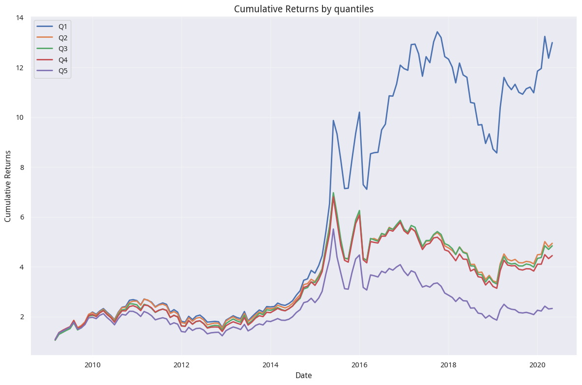
Although we only used 50 stocks for the backtest, changing the universe parameter to 3000 would still yield excellent results.
The results look quite good! They are almost consistent with what the research report stated. Of course, if you are familiar with the basic theory of factor testing, you would know that this factor is actually a reverse factor—it serves as an excellent "topping indicator."
Why Our Results Are Better
Looking at the return chart, our results are better than those in the research report for three reasons. First, `moonshot` does not calculate transaction fees. Second, we cannot precisely reproduce the universe used in the research report’s backtest. Third, fully reproducing the research report is difficult because many technical details are omitted when writing the report.Let’s now examine the Williams lower shadow moving average factor.
from moonshot import Moonshot
def calculate_williams_r_ratio(bars):
"""
计算变种威廉指标
"""
high = bars['high']
low = bars['low']
close = bars['close']
wr_up = high - close
wr_down = close - low
rolling_wr_up = wr_up.rolling(5).mean()
rolling_wr_down = wr_down.rolling(5).mean()
# 与蜡烛上下影线的默认值不同,0.5 更能表明无信号的含义
wr_up_ratio = pd.Series(0.5, index=bars.index)
wr_down_ratio = pd.Series(0.5, index=bars.index)
mask = rolling_wr_up > 1e-8
wr_up_ratio[mask] = wr_up[mask] / rolling_wr_up[mask]
mask = rolling_wr_down > 1e-8
wr_down_ratio[mask] = wr_down[mask] / rolling_wr_down[mask]
return wr_up_ratio, wr_down_ratio
def calc_wr_down_factor(barss, win = 20):
wr_down = (barss.groupby("asset", group_keys=False)
.apply(lambda x: calculate_williams_r_ratio(x)[1])
.sort_index())
return calc_monthly(wr_down, "mean", win)
start = datetime.date(2009, 1, 1)
end = datetime.date(2020, 4, 30)
barss = load_bars(start, end, 50)
factor = calc_wr_down_factor(barss, 20)
ms = Moonshot()
ms.backtest(factor, barss)
ms.plot_cumulative_returns_by_quantiles()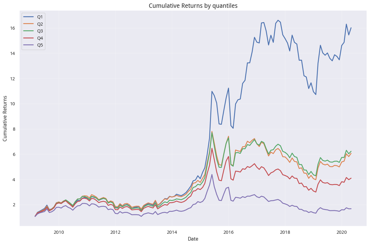
This chart confirms what the research report stated: the Williams lower shadow moving average factor is also a strong stock selection factor. However, did you notice? The smaller the lower shadow mean, the higher the probability of future price increases. Isn’t this counter-intuitive? Furthermore, this seems inconsistent with the statement made at the beginning of the research report.
At the start of the report, the author mentioned that a longer Williams lower shadow indicates stronger buying interest and bullish outlook, while a shorter one suggests bearishness. They cited examples of the Shanghai Composite Index on February 3 and 4, 2020. What’s going on here?
tip
Before reading this research report, my intuitive experience suggested that a longer lower shadow often means buying pressure exceeds selling pressure, making a reversal more likely. However, seeing these results made me re-evaluate my experience. My experience was partially correct; but this also highlights the clearest divide between subjective and quantitative approaches: our subjective memory retains only a few happy or painful moments, while actively "forgetting" vast amounts of ordinary days. Statistically, however, those ordinary days, under the effect of compound interest, may be the signposts leading us to the peak of our lives.Conversely, the fifth group has the highest factor values, meaning the stock frequently closes near its highest price. This may imply higher "chasing risk" and limited upside potential.
UBL Factor
So, what is the effect of combining these two factors as proposed in the research report?
def calc_ubl_factor(barss, win=20):
from scipy.stats import zscore
up_std = calc_candle_up_std_factor(barss, win)
wr_down = calc_wr_down_factor(barss, win)
# 截面 zscore
z_scored_up_std_factor = up_std.groupby("date").transform(
lambda x: zscore(x, nan_policy="omit")
)
z_scored_wr_down = wr_down.groupby("date").transform(
lambda x: zscore(x, nan_policy="omit")
)
return z_scored_up_std_factor + z_scored_wr_down
start = datetime.date(2009, 1, 1)
end = datetime.date(2020, 4, 30)
barss = load_bars(start, end, universe=50)
factor = calc_ubl_factor(barss, 20)
ms = Moonshot()
ms.backtest(factor, barss)
ms.plot_cumulative_returns_by_quantiles()By changing universe = 50 to 3000 in the code, we obtained similar group results.
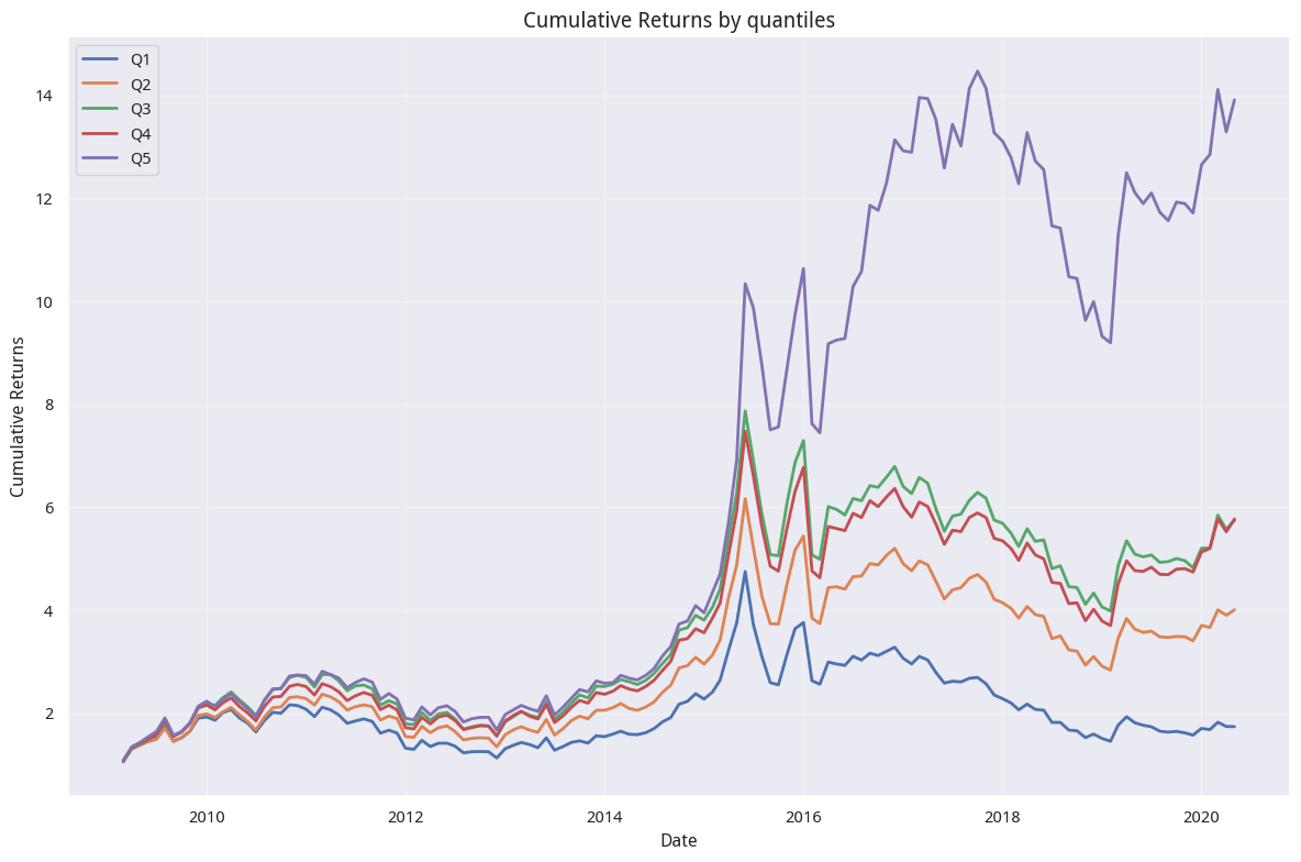
From the perspective of layered cumulative returns, it seems similar to that of the individual factors (i.e., the separate candlestick upper shadow standard deviation or the standalone Williams lower shadow mean). However, the key point is that the long-short combination exhibits very robust characteristics:
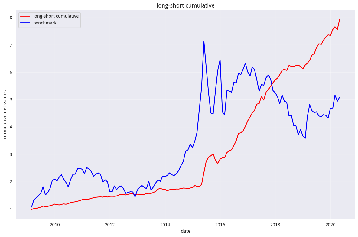
In investing, we prefer "calm lakes in spring" over "distant peaks." We love these net value curves that look up at the stars at a 45-degree angle.
The research report only backtested until April 2020. What happened later? You can read the notebook version of this article on the Quantide Research Platform, adjust the parameters, and run it yourself. You might be surprised.
Final Thoughts: On Cross-Sectional Z-Score
According to the research report, when calculating the UBL factor, one should perform cross-sectional z-score processing on the up_shadow_std factor and the wr_down_mean factor daily. We implemented this requirement in our example.
But is this truly necessary?
First, we must note that the default behavior of z-score has NaN propagation. That is, if any asset’s factor value is NaN in the input factors for a given day, the z-scored calculated values for all assets on that day will become NaN, rendering subsequent calculations meaningless.
Therefore, if we must use z-score, we must handle this situation properly. This is why, in the example above, we passed lambda x: zscore(x, nan_policy='omit') into the transform function.
Second, z-scoring factors does not change the ranking of factors within the same day. Since factor group return calculations are performed based on this ranking afterward, cross-sectional z-scoring here may simply be a habit, at least having no impact on the calculation of group cumulative returns.