Dragon Taming: Engineering a Candlestick Factor from Folklore to Quant

"Three incense sticks on the head, death or total loss." This Chinese stock proverb suggests that if three long upper shadows appear at high levels, the stock price is likely to drop in the short term. The rationale is that upper shadows indicate significant selling pressure above. Can this adage be validated statistically? A research report from Dongwu Securities explores this very question.

The report offers a valuable conclusion: the utility of shadows depends not on the shadows themselves, but on how you use them. Starting from common K-line patterns, the report connects to the Williams %R indicator and employs basic statistical theory for modeling and extension. Both the conclusions and the research methodology offer significant reference value for quantitative researchers.

Factor Principle

Shadows are essentially traces of failed attempts to push the stock price to the day’s high (or low). The high and low prices represent the outcome of the day’s long-short博弈 (game), reflecting the true support and resistance recognized by the market. This viewpoint is also mentioned in an Everbright Securities research report (the RSRS factor paper) and is a widely accepted view in the industry. Approaching this from different angles and using different modeling methods yields distinct factors.

Starting from the traditional definitions of upper and lower shadows, and after comparing them with the Williams %R indicator, the authors creatively treat the Williams %R itself as a type of 'shadow.' They then apply mean normalization to the raw shadows (including both traditional and Williams shadows) and construct four factors using rolling means and rolling standard deviations, which are subsequently tested.

After factor testing, they found that the standardized candlestick upper shadow and the mean-normalized Williams lower shadow exhibited strong stock-selection power. Consequently, they combined these two factors into a new factor, named UBL.

The final backtest results (from 2009 to April 30, 2020) are as follows:

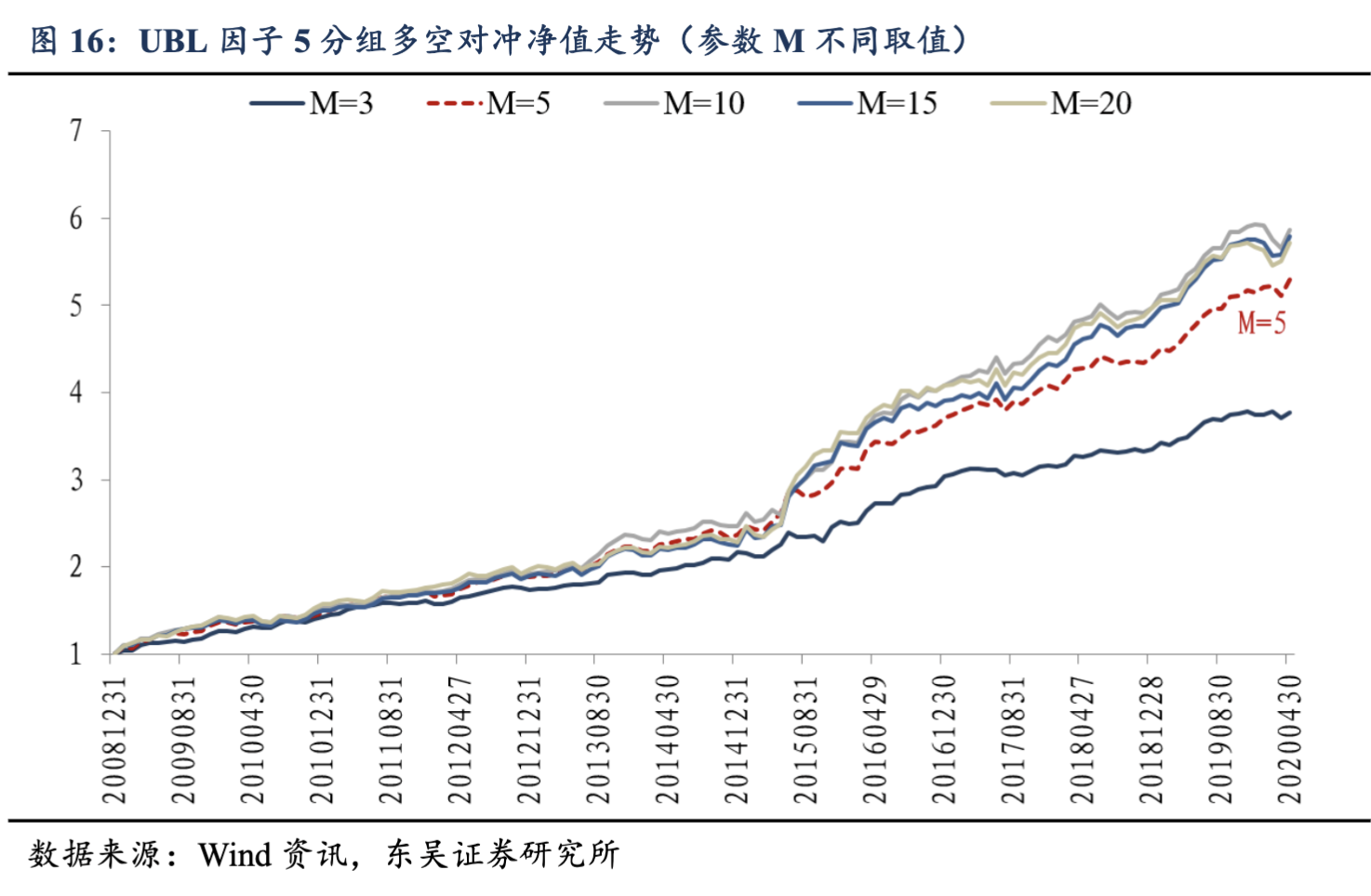
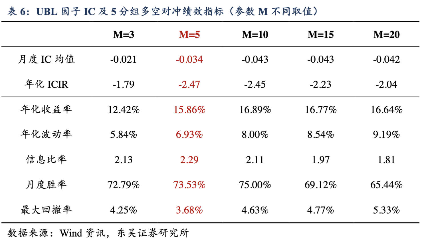
Below, we implement this factor.

Factor Construction

According to the report, the factor construction process is as follows:

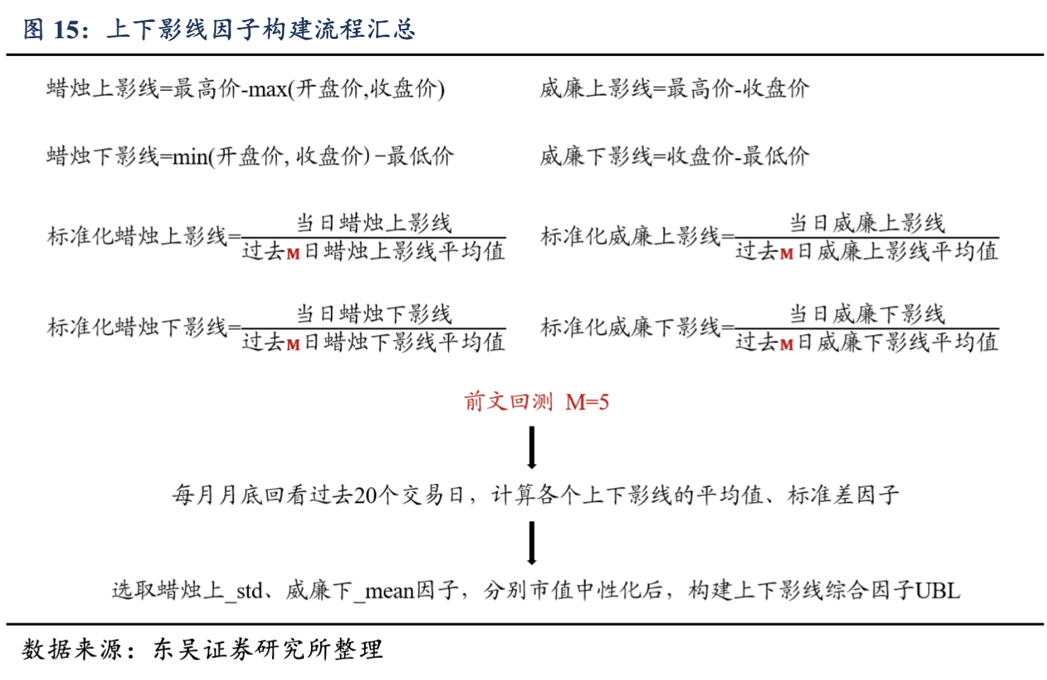
Following the diagram, we first implement the upper and lower shadows.

The code below calculates the upper and lower shadows:

1234567891011121314151617181920212223242526def calculate_shadow_ratio(bars):
    """Calculate upper and lower shadow factors (normalized)
    
    Per the report, the standardized candlestick upper shadow is the daily upper shadow divided by the 5-day mean of upper shadows. The standardized candlestick lower shadow is calculated similarly.
    """
    high = bars['high']
    low = bars['low']
    open_price = bars['open']
    close = bars['close']

    # To avoid division by zero, we use a trick: masking out calculations where division by zero might occur.
    # When calculation is impossible, we set the value to 0, indicating no signal.
    up_shadow_ratio = pd.Series(0, index=bars.index)
    down_shadow_ratio = pd.Series(0, index=bars.index)

    up_shadow = high - np.maximum(open_price, close)
    rolling_up_shadow = up_shadow.rolling(5).mean()
    mask = rolling_up_shadow > 1e-8
    up_shadow_ratio[mask] = up_shadow[mask] / rolling_up_shadow[mask]

    down_shadow = np.minimum(open_price, close) - low
    rolling_down_shadow = down_shadow.rolling(5).mean()
    mask = rolling_down_shadow > 1e-8
    down_shadow_ratio[mask] = down_shadow[mask] / rolling_down_shadow[mask]

    return up_shadow_ratio, down_shadow_ratio

Calculating the upper and lower shadows is straightforward. However, per the report, the critical step is 'standardization': dividing by the 5-day mean of the shadows to eliminate dimensional differences across different assets.

From the formula, we inevitably face a division-by-zero issue: if a stock has no shadows for the past 5 days, the 5-day mean of the shadows will be zero. How do we avoid this?

Division-by-zero errors are common in quantitative modeling, and solutions vary by scenario. Here, we use a small trick worth noting.

The report authors argue that variants of the Williams %R indicator—specifically, the difference between the closing price and the high/low prices (after standardization)—also reflect selling pressure and buying momentum, thus holding signal significance.

Its calculation method is:

12345678910111213141516171819202122232425def calculate_williams_r_ratio(bars):
    """
    Calculate variant Williams %R
    """
    high = bars['high']
    low = bars['low']
    close = bars['close']
    
    wr_up = high - close
    wr_down = close - low

    rolling_wr_up = wr_up.rolling(5).mean()
    rolling_wr_down = wr_down.rolling(5).mean()

    # Unlike the default value for candlestick shadows, 0.5 better signifies 'no signal'
    wr_up_ratio = pd.Series(0.5, index=bars.index)
    wr_down_ratio = pd.Series(0.5, index=bars.index)

    mask = rolling_wr_up > 1e-8
    wr_up_ratio[mask] = wr_up[mask] / rolling_wr_up[mask]

    mask = rolling_wr_down > 1e-8
    wr_down_ratio[mask] = wr_down[mask] / rolling_wr_down[mask]

    return wr_up_ratio, wr_down_ratio

Monthly Factor Calculation

The report applies multiple transformations to the factors. So far, we have only performed the first transformation: 'standardization.' The actual factors are derived from the mean or standard deviation calculated at the end of each month.

This operation is generalizable, so we extract it into a function. This section employs several pandas operation techniques.

1234567891011121314151617181920212223def calc_monthly(daily_factor, aggfunc, win=20):
    dates = daily_factor.index.get_level_values('date').unique().sort_values()
    month_ends = dates.to_frame(name = "date").resample('BME').last().values

    dfs = []

    for date in month_ends:
        date_ts = pd.Timestamp(date.item())
        iend = dates.get_loc(date_ts)
        istart = max(0, iend - win + 1)
        start_ = pd.Timestamp(dates[istart])
        end_ = date_ts
        window_data = daily_factor.loc[start_: end_]

        df = (window_data.groupby(level="asset")
                        .agg(aggfunc)
                        .to_frame("factor")
        )
        df["date"] = date_ts
        dfs.append(df)

    df = pd.concat(dfs)
    return df.set_index(["date", df.index]).sort_index()

In this step, we implement the calculation of a monthly factor at the end of each month, using win as the data window. The report uses mean and standard deviation as aggregation functions. To allow for the exploration of more factors, we allow the aggregation function to be passed as a parameter here.

With this function, we can immediately calculate the candlestick upper_mean, candlestick upper_std, and other factors proposed at the beginning of the report:

123456def calc_candle_up_std_factor(barss, win = 20):
    up_shadow = (barss.groupby("asset", group_keys=False)
                      .apply(lambda x: calculate_shadow_ratio(x)[0])
                      .sort_index())

    return calc_monthly(up_shadow, "std", win)

The factor data we currently have looks roughly like this:

Similarly, we can calculate the Williams lower_mean factor:

123456def calc_wr_down_factor(barss, win = 20):
    wr_down = (barss.groupby("asset", group_keys=False)
                    .apply(lambda x: calculate_williams_r_ratio(x)[1])
                    .sort_index())

    return calc_monthly(wr_down, "mean", win)

UBL Factor

According to the report, calculating the UBL factor requires market-cap neutralization of the aforementioned monthly factors, followed by cross-sectional standardization of the two factors, and finally summing them.

Here, we omit the market-cap neutralization step and proceed directly to cross-sectional z-score normalization.

12345678up_std = calc_candle_up_std_factor(barss, win)
wr_down = calc_wr_down_factor(barss, win)

# Cross-sectional z-score
z_scored_up_std_factor = up_std.groupby("date").transform(zscore)
z_scored_wr_down = wr_down.groupby("date").transform(zscore)

return z_scored_up_std_factor + z_scored_wr_down

123456789101112131415161718
We can verify the correctness of the factor calculation process using the following data.

```python
dates = pd.bdate_range('2019-01-01', '2019-01-31')
cols = ["open", "high", "low", "close"]
df1 = pd.DataFrame([(2, 3, 1, 2)] * len(dates), index=dates, columns=cols)
df1["asset"] = "A"

df2 = pd.DataFrame([(2, 3, 0, 0)] * len(dates), index=dates, columns=cols)
df2["asset"] = "B"

barss = pd.concat([df1, df2]).set_index("asset", append=True)
barss.index.set_names(["date", "asset"], inplace=True)
barss.sort_index(inplace=True)

display(calc_candle_up_std_factor(barss, 20))
display(calc_wr_down_factor(barss, 20))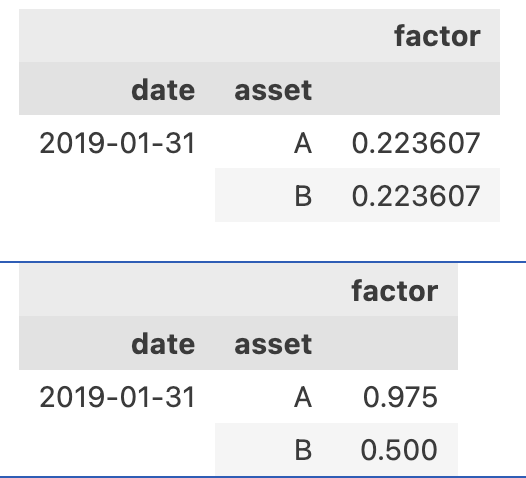

The standard deviation factor for the upper shadow yields 0.22367 for both assets A and B.

For simplicity, the upper shadow values for assets in our test data are set to identical values. Why is the standard deviation not zero? This is because, during the calculation, the first few trading days had missing values due to the sliding window (win=5) being insufficient. These missing values were filled with zeros. The calculation of the standard deviation involving these zeros and subsequent non-zero values resulted in a standard deviation of 0.22367.

Conclusion

In this article, we used a very simple example to explain how to read research reports and translate them into code. After understanding basic terminology (such as mean, standard deviation, cross-sectional standard deviation, and z-score), the remaining task is to pay attention to details in engineering practice, such as how to handle missing values and assign appropriate default values. This part is often less discussed in research reports and usually stems from your trading experience and understanding of factors.

Additionally, this article mentions differences in the implementation of basic concepts across different Python libraries. For example, the calculation of standard deviation differs between Pandas and Numpy. Typically (when using standard deviation merely as a measure of error), this difference can be ignored. However, once you use it as a factor, you must pay attention to this discrepancy.

Quantitative trading is not just about having an idea and automatically implementing it. The success of quantitative trading strategies requires both 'genius'-level creativity and innovation, and the ability to delve into every detail to implement it correctly. This often requires systematic training. KuangTi's quantitative courses are renowned for their rigorous and systematic content. If you are looking for such a course, we strongly recommend studying KuangTi's 'Quantitative Twenty-Four Lessons' and 'Factor Mining and Machine Learning Strategies' courses.

This article is part of a series. In the next article, we will conduct factor backtesting to verify the report's conclusions. Please follow and subscribe for timely updates. The source code for this article (and subsequent articles) is available for reading and running on the Quantide Research platform.