Why Every Quant Should Use DuckDB

In my last note, I showed how to manipulate DataFrames with SQL in DuckDB. I also highlighted its unique AsOf Join — incredibly handy for quants who constantly need to align multi-timeframe market data. But DuckDB has a lot more to offer.

• A full SQLite replacement, with a command set that even goes beyond Postgres
• Excellent usability
• A performance beast

Yet another gem from the sparsely populated Netherlands — the cold north surprises again. Tech breakthroughs clearly aren't about headcount.

SQLite is extremely lightweight, storing data in memory or a single file with none of the complex server setup other databases require. It's the most widely deployed database in the world — but that may change: functionally, DuckDB not only covers everything SQLite does, its SQL dialect is arguably even richer than Postgres. On performance, SQLite isn't even in the same league — in fact, on joins and group-bys over large datasets, H2O.ai benchmarks put DuckDB at #1, ahead of star players like ClickHouse and Polars!

Replacing SQLite

When using SQLite, especially for unit tests, we often use an in-memory database. DuckDB supports that too:

123import duckdb

duckdb.connect(":memory:")

Swap ":memory:" for a file path and you're connected to a file-backed database. No different from SQLite here.

Both SQLite and DuckDB have the concept of rowid. In DuckDB, rowid is a pseudo-column:

12345-- duckdb中的rowid无须声明，可直接使用

CREATE TABLE t (id INT, content STRING);
INSERT INTO t VALUES (42, 'hello'), (43, 'world');
SELECT rowid, id, content FROM t;

If a row is deleted, its rowid is recycled and may be reused later, so rowid is not unique and shouldn't be used as a row identifier.

For auto-increment IDs, SQLite lets you declare a primary key with the AUTOINCREMENT keyword, while DuckDB takes one extra step — you first create a sequence:

12345678CREATE SEQUENCE seq_personid START 1;

CREATE TABLE Persons (
    Personid integer primary key DEFAULT nextval('seq_personid'),
    Name varchar(255) not null,
);

insert into Persons values ('Aaron')

In other words, create a sequence first, then declare the primary key's default as nextval(). When inserting, just omit PersonId.

Building Queries Incrementally

SQL is powerful, but it can get complex and verbose. Anyone familiar with pandas knows DataFrame queries can be complex too — but you can build them step by step, inspecting intermediate results to stay correct, which makes pandas much easier to learn.

DuckDB borrows that idea. Its Python client offers a Relational API for exactly this workflow.

12r = duckdb.sql("from range(1000000000) tbl(id)")
r.show()

The first line builds a relation — with no SELECT! That's DuckDB's shorthand for SQL. Once you get used to it, the traditional SELECT * FROM ... feels downright verbose.

The first line doesn't execute anything; evaluation only happens when you call r.show().

12r = duckdb.sql("from range(10000) tbl(id) select id, cast (id as varchar) as str_id")
r.filter("id > 20 and str_id like '%1'").limit(3).show()

It feels a lot like pandas, except the expressions are SQL and the method names track SQL keywords closely.

In the first line, SELECT comes after FROM — a DuckDB syntax innovation. In the second line, the expression is pure SQL. As I covered last time, pandas doesn't support this syntax.

If you're more comfortable with pandas syntax, couldn't you just load data into a DataFrame (via read_csv, read_sql) and query it there? Yes and no. pandas can't handle data larger than memory. When datasets get big, DuckDB's API really shines.

The example shows string matching. DuckDB has rich function support, including string slicing and regex matching. This is a fairly specialized case, though, so I haven't seen performance benchmarks for it.

Another sweet spot for the Relational API is JOIN and INTERSECT:

1234import duckdb
r1 = duckdb.sql("FROM range(5) tbl(id)").set_alias("r1")
r2 = duckdb.sql("FROM range(10, 15) tbl(id)").set_alias("r2")
r1.join(r2, "r1.id + 10 = r2.id").show()

The syntax here is concise and readable (even clearer than pandas joins). Whether you're building subqueries or CTEs, plain SQL gets verbose and error-prone — the Relational API simplifies it all and makes debugging from intermediate results easy. Here's a subquery example:

1duckdb.sql("SELECT t FROM (SELECT unnest(generate_series(41, 43)) AS x, 'hello' AS y) t where t.x > 42")

We can easily break it down into:

123r1 = duckdb.sql("SELECT unnest(generate_series(41, 43)) AS x, 'hello' AS y")
r2 = duckdb.sql("from r1").filter("x>42")
r2

So if you're a SQL expert, you can still hand DuckDB complex SQL directly; if you can only write short SQL snippets, you can still assemble them into complex queries via the Relational API.

In quant work, data is often time-series in nature, and we constantly compute rolling-window stats like min/max and averages. pandas gives you rolling() for that. In DuckDB, you do it with OVER and a family of window functions.

Take power-plant generation data as an example:

The following query computes a 7-day moving average of daily output:

123456789SELECT "Plant", "Date",
    avg("MWh") OVER (
        PARTITION BY "Plant"
        ORDER BY "Date" ASC
        RANGE BETWEEN INTERVAL 3 DAYS PRECEDING
                  AND INTERVAL 3 DAYS FOLLOWING)
        AS "MWh 7-day Moving Average"
FROM "Generation History"
ORDER BY 1, 2;

You can also define named windows with WINDOW so they can be reused for better performance:

12345678910111213141516SELECT "Plant", "Date",
    min("MWh") OVER seven AS "MWh 7-day Moving Minimum",
    avg("MWh") OVER three AS "MWh 3-day Moving Average",
FROM "Generation History"
WINDOW
    seven AS (
        PARTITION BY "Plant"
        ORDER BY "Date" ASC
        RANGE BETWEEN INTERVAL 3 DAYS PRECEDING
                  AND INTERVAL 3 DAYS FOLLOWING),
    three AS (
        PARTITION BY "Plant"
        ORDER BY "Date" ASC
        RANGE BETWEEN INTERVAL 1 DAYS PRECEDING
        AND INTERVAL 1 DAYS FOLLOWING)
ORDER BY 1, 2;

Notice the PARTITION syntax above. Every OVER clause (windowing) implies a single partition when PARTITION BY is omitted, or multiple partitions when it's present. Within each partition, RANGE, PRECEDING, FOLLOWING and friends define sliding frames, and aggregations run over those frames.

The QUALIFY Clause

This is a relatively new SQL clause, introduced years ago by Teradata and later adopted by Oracle, Snowflake, and BigQuery. It solves a classic problem: how do you take the top-N values per group (or rows matching some other window condition) along with the full row?

Where pandas is available, this is easy:

123df = pd.DataFrame({'id':[1,1,1,2,2,2,2,3,4], 'value':[1,2,3,1,2,3,4,1,1]})

df.groupby('id')["value"].nlargest(2)

Output:

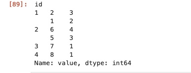
With other conditions, you can filter after groupby using apply with a lambda.

In standard SQL, the same task requires a subquery — first select the qualifying row IDs per group, then fetch the full rows from the base table. It's clunky. With QUALIFY, it collapses to:

1234df = pd.DataFrame({'id':[1,1,1,2,2,2,2,3,4], 'value':[1,2,3,1,2,3,4,1,1]})

sql = "select id, value from df qualify row_number() over (partition by id order by value desc) <=2 order by value"
duckdb.sql(sql).sort("id")

This query returns the two largest values per id, with full rows. OVER defines the window: PARTITION BY id splits the table into independent sub-tables, ORDER BY value sorts within each, and row numbers are assigned per partition. Finally, QUALIFY keeps rows numbered 1-2 — exactly what we want.

DuckDB's Dutch Dialect

DuckDB streamlines some of standard SQL's verbosity — like the FROM tbl shorthand we saw earlier that drops SELECT *.

In quant research, a factor library is often one very wide table with similarly named columns. For example, you might store 30-minute, daily, and weekly RSI as separate factor columns.

When you want all three at once, use its dynamic column selection. For example, SELECT COLUMNS('RSI_*') FROM alpha101

If all your RSI factors share the RSI prefix with different suffixes, one expression grabs them all.

DuckDB also supports chaining scalar functions, for example:

12345678SELECT 
     ('Make it so')
          .UPPER()
          .string_split(' ')
          .list_aggr('string_agg','.')
          .concat('.') AS im_not_messing_around_number_one;
-- 输出
-- MAKE.IT.SO.

Many more fun features are covered in their blog post, Even Friendlier SQL with DuckDB.

What Is DuckDB, Really?

DuckDB connects to many databases and data sources — in plenty of examples you'll see it analyzing CSV and Parquet files directly. Used this way, you're really just using its analytical engine.

To get the most out of DuckDB's features and performance, it's best to import data into its native file format — a file-based database. It's columnar and compressed, much like Parquet, but goes further: it can hold multiple tables and views, supports ACID, and allows schema changes and added columns without rewriting the file. As a rule of thumb, importing Parquet files into DuckDB costs about 20% extra disk space.

Of course, DuckDB has limits too. For instance, multi-process writes aren't supported.

Performance

For quants, reason #2 to use DuckDB (#1 being AsOf Join) is performance. In H2O.ai's leaderboard for the most demanding GROUP BY and JOIN workloads — from 0.5GB to 5GB and 50GB — DuckDB ranks first, followed by ClickHouse and Polars. We'll still use ClickHouse regardless; the two cover different use cases.

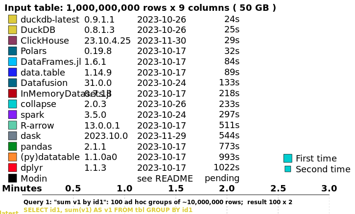
That said, the standard database benchmark is TPC-DS. According to tests by Fivetran's CEO, DuckDB beats the best commercial databases when the stored files are under 250GB, but falls behind on a 1TB dataset (on 32 cores with 128GB RAM).

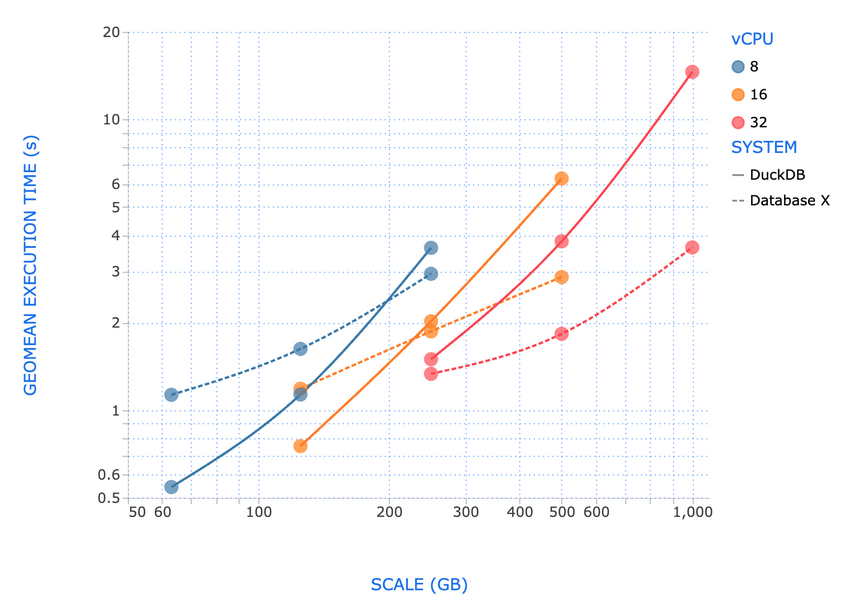
The takeaway: DuckDB can at least handle around 1TB, but its sweet spot is under 100GB — so it's probably still not the right store for tick-level market data.

Using DuckDB in Notebooks

In notebooks you can query directly with DuckDB's Python API. Alternatively, the JupySQL extension lets you run SQL and visualize results.

Install JupySQL with:

1pip install jupysql

Before using JupySQL, load the extension:

1%load_ext sql

Next, connect. For file storage:

1%sql duckdb:///path/to/fild.db

Then you can use cell magic in subsequent cells:

12345678%%sql

SELECT
    schema_name,
    function_name
FROM duckdb_functions()
ORDER BY ALL DESC
LIMIT 5

This is a bit more convenient than the Python API, since you can indent and break lines freely. With SQLite I often used SQLite Browser to inspect generated tables, but JupySQL alone can cover that workflow.

Conclusion

As a quant, I strongly recommend DuckDB as your personal database tool. It fully replaces and outperforms SQLite3. Built on columnar storage and vectorized execution, it even beats ClickHouse and Polars on these workloads.

In short: if you need to analyze 100GB of data on a 16GB machine, DuckDB is the answer.