Give Pandas a Partner: Query DataFrames with SQL & DuckDB

If you know some SQL, querying in pandas can feel tedious.

In this post, we'll find Pandas a companion: use SQL where SQL is handy, and native pandas where native is handy.

So who will this companion be?

A DataFrame is essentially a table. pandas provides many methods to query a DataFrame, and they often map directly to SQL queries, for example:

1. Select a few columns from a table. The equivalent SQL is:

   1SELECT total_bill, tip, smoker time from tips;

   In pandas, the syntax is actually a bit more concise:

   1tips[["total_bill", "tip", "smoker", "time"]]

2. Filter by conditions. When you have many conditions or need fuzzy matching, pandas is not as concise as SQL:

   1select * from tips where time like 'Dinner%' and tip > 5;

   SQL reads almost like natural language. In pandas, you have to write:

   1tips[(tips["time"].str.find("Dinner") == 0) & (tips["tip"] > 5)]

   The string-operation syntax may be more powerful, but it is not as intuitive as SQL. The logical operators for multiple conditions are also less readable than AND. To query for nulls, in SQL you write:

   1select * from frame where col2 is NULL;

   In pandas, you need to use isna() or notna().

3. Aggregation is also routine in data processing.

   1select smoker, day, count(*), avg(tip) from tips group by smoker, day;

   In pandas, you would write:

   1tips.groupby("day").agg({"tip": "mean", "day": "size"})

   The syntax is less intuitive, but fairly compact.
4. Joining tables. SQL has powerful JOIN and UNION syntax. In pandas, three functions cover this area: join, merge, and concat. join defaults to a left join on columns, merge defaults to an inner join on columns, and concat defaults to an outer join on rows. Designing multiple APIs for similar jobs is part of what makes pandas harder to learn and remember. The difference between join and merge is that join can handle multiple tables at once but only works on the index, while merge handles only two tables at a time but can join on any columns. concat works row-wise by default, joins only on the index with inner and full (default) joins, and can operate on multiple DataFrames at once.

In addition, we need sorting, limiting the number of rows returned, and pagination. pandas has corresponding functions for all of these, but if you already know SQL well, the pandas APIs are hard to map one-to-one to SQL.

Now, let's see how we can treat a DataFrame as a database table and query it with SQL. If we can pull this off, many queries will become much simpler.

The Built-in query Method

Surprisingly, pandas already ships with a query method that lets you query pandas as if you were running SQL.

The function signature is:

12345DataFrame.query(expr, *, inplace=False, **kwargs)

# 最简单的查询。这将返回满足列A大于列B的所有行
# 类似于df[df.A > df.B]
df.query('A > B')

With this query method, we can simplify queries. Let's first generate a dataset:

12345import pandas as pd

from pandas.util.testing import makeMixedDataFrame
df = makeMixedDataFrame()
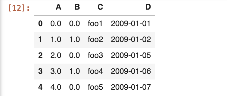
df.head()

Here we use makeMixedDataFrame from the testing package to generate a test DataFrame. makeMixedDataFrame produces a DataFrame with various dtypes, except None. If you want a test DataFrame with missing values, you can use makeMissingDataframe.

The resulting DataFrame looks like this:

Now, let's run a query:

1df.query("A>3 and B <= 1.0")

This returns the 4th record of the original dataset.

Note that the query expression only looks like SQL — it isn't SQL syntax. Its first argument, the expr argument, is a Python expression, not a SQL statement. In the sample data above, if we want to find rows where column C contains 'foo', we can't use SQL's LIKE keyword. Instead, we have to do this:

1df.query("A>3 and C.str.find('foo')!=-1")

This is basically back to DataFrame-style querying, except that we are allowed to use AND as the logical operator. The main reason to use query is speed. If numexpr is installed in your environment, query will use numexpr to accelerate computation by default, and on DataFrames with over 1 million rows it can be quite a bit faster than the various DataFrame filter methods.

pandasql

The first attempt to bring SQL querying to pandas was pandasql.

1! pip install pandasql

Now we can query with full SQL syntax:

1234from pandasql import sqldf
pysqldf = lambda q: sqldf(q, globals())
pysqldf("select A, C, count(*) as count 
        from df group by B limit 2;")

Grouping, limiting rows, and renaming columns in one go — this example shows the power of SQL nicely.

But pandasql has a significant problem: it hasn't been updated for a long time. I mentioned SQLAlchemy version-management issues in my book Python for Large Projects (《Python能做大项目》), and the same problem shows up here. When you install pandasql today, it pulls in SQLAlchemy 2.0. That version causes the following error:

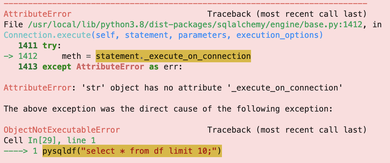
To fix it, you'd have to downgrade to SQLAlchemy 1.4.46. But since so many other libraries (including Pandas) depend on newer versions of SQLAlchemy, that fix only creates new chaos.

Let's keep looking for a new solution. That solution is DuckDB.

DuckDB

Pandas is the plural of panda, and the partner we've found for it is called Duck — a match made in heaven.

DuckDB is an in-process OLAP database management system. It speaks SQL natively, but integrates very tightly with DataFrame libraries like Pandas, Polars, and Vaex. It is written in C++, but offers Python, R, and even newer wasm interfaces. What we care about most here is the ability to query directly against a DataFrame as the data source.

12345678import duckdb
import pandas

# Create a Pandas dataframe
my_df = pandas.DataFrame.from_dict({'a': [42]})

# query the Pandas DataFrame "my_df"
results = duckdb.sql("SELECT * FROM my_df").df()

It's even more concise than pandasql. We don't need to bind the current environment's globals for DuckDB — DuckDB can automatically find my_df!

Learning DuckDB is very easy. Because as long as you know SQL, you've already mastered almost all of it. That's the magic.

Still, we can show a more powerful example that comes up all the time in our quant workflow.

As-of Join

As a developer of an open-source quant framework, this problem haunted me for a long time:

Give me the value of the adjust factor as of this time.

With DuckDB, implementing this becomes very simple. To demonstrate a real-world scenario, we'll use the data source from the Quant 24 Lessons environment:

12345from coursea import *

await init()

code = "000001.XSHE"

12345678910end_day = datetime.date(2023, 6, 14)
end_time = datetime.datetime(2023, 6, 14, 15)

# 获取2天的日线并转换成DataFrame
day_bars = await Stock.get_bars(code, 2, FrameType.DAY, end=end_day)
day_bars = pd.DataFrame(day_bars)

# 获取对应日期下的60分钟线，并转换为DataFrame
min_bars = await Stock.get_bars(code, 8, FrameType.MIN60, end=end_time)
min_bars = pd.DataFrame(min_bars)

Of course, the minute bars you get via zillionare-omicron are already adjusted for you. For demonstration purposes, here we rebuild them with DuckDB's asof join and compare against zillionare's result:

1234567import duckdb

sql = """SELECT m.frame, m.close, d.factor
FROM min_bars m ASOF left JOIN day_bars d
 on m.frame >= d.frame;"""

duckdb.sql(sql)

The output is in DataFrame format, as follows:

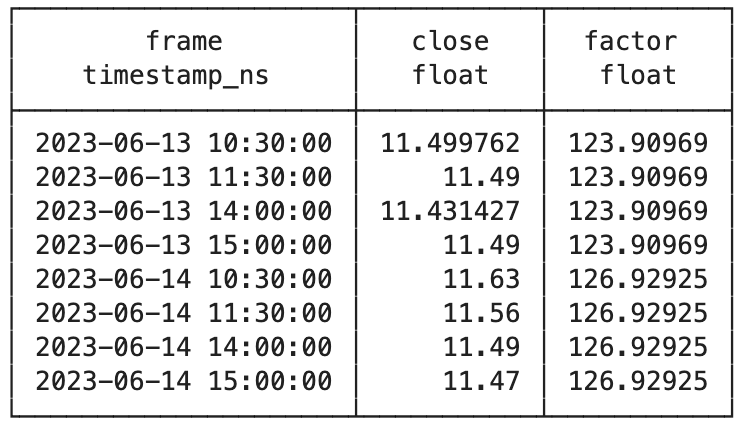
We can see an adjustment happened on June 14, 2023. Next, let's compare against the data fetched from zillionare-omicron to check whether the adjustment time, factor, and close price all match:

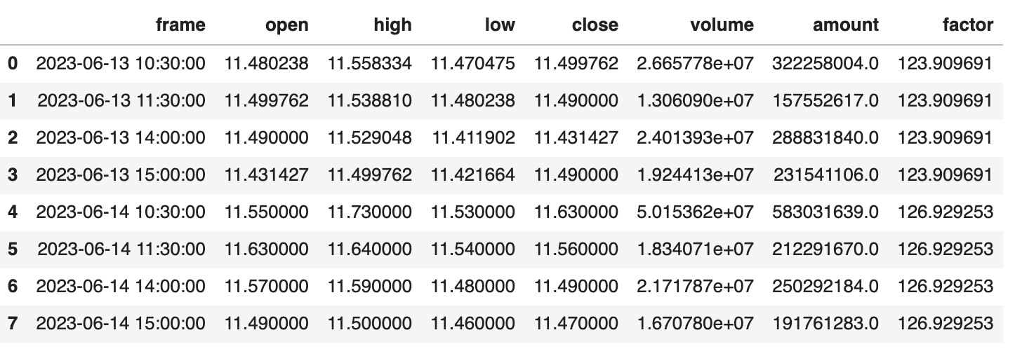
As you can see, the two results match. But the DuckDB implementation is quite a bit faster than zillionare.

This post is mainly about how to enhance — or simplify — pandas DataFrame queries with SQL. But DuckDB can do far more than that. In a previous post we mentioned that to store massive amounts of data you can use pyarrow + parquet, with pyarrow handling the queries. But if you prefer SQL-based queries, you can use DuckDB instead.

Starting with pandas and ending with a recommendation of DuckDB + parquet — does that count as an O. Henry-style twist?