
Moonshot Backtest: Dividend Yield Factor Alpha in China A-Shares
abstract
1. How to retrieve dividend yield data from Tushare and leverage its pagination mechanism to accelerate data retrieval? 2. How to implement screening based on dividend yield? A detailed comparison of `pandas` `transform` vs. `apply` methods. 3. The alpha generated by dividend yield data.Now, we enter the second phase: gradually adding factors and conducting backtests.
Our first addition is the dividend yield factor, which we will use to screen the stock universe.
Fetching Dividend Yield
In Tushare, there are two approaches to obtaining dividend yield data. The first is via the daily_basic interface. The second involves fetching the per-share dividend via the dividend interface and dividing it by the share price.
Here, we demonstrate only the first method. However, when we later implement screening for companies with two consecutive years of dividends, we will show how to use the dividend interface.
The daily_basic interface retrieves common daily data indexed by date, such as closing price, turnover rate, P/E ratio, market cap, and approximately 15 other columns. Its signature is as follows:
def daily_basic(
ts_code: str, trade_date: str, start_date: str, end_date: str
) -> pd.DataFrame:
passEither ts_code or trade_date is required. Like most Tushare functions, it has a record limit, currently set at 6,000 records. This allows fetching about 25 years of data for a single stock or one day’s data for all stocks in a single request.
attention
The record limit per request may depend on your account tier. The 6,000-record limit shown here applies to accounts with 5,000+ points.# example-1
def fetch_dv_ttm(start: datetime, end: datetime) -> pd.DataFrame:
pro = ts.pro_api()
cols = "ts_code,trade_date,dv_ttm,total_mv,turnover_rate,pe_ttm"
dfs = []
for dt in pd.bdate_range(start, end):
dtstr = dt.strftime("%Y%m%d")
df = pro.daily_basic(trade_date=dtstr, fields=cols)
dfs.append(df)
return pd.concat(dfs)
df = fetch_dv_ttm(datetime.date(2019, 10, 8), datetime.date(2019, 10, 12))
dfIt takes approximately 0.5 seconds to fetch one day’s data. Consequently, fetching a full year’s data takes about 2 minutes.
Screening by Dividend Yield
We now implement a screen to select the top 500 stocks by dividend yield daily, then backtest this universe using Moonshot to assess its inherent value.
import tushare as ts
from helper import qfq_adjustment
from fetchers import fetch_bars
from store import ParquetUnifiedStorage, CalendarModel
from moonshot import Moonshotfrom moonshot import Moonshot
def dividend_yield_screen(data: pd.DataFrame, n: int = 500)->pd.Series:
"""Dividend yield screening method
Ranks dividend yield monthly, selects the top n stocks, marks them as 1,
and performs a logical AND with the existing flag.
Args:
n: Number of stocks to select monthly, default 500
"""
logger.info("Starting dividend yield screening...")
if 'dv_ttm' not in data.columns:
raise ValueError("dv_ttm column not found in data; screening cannot be applied")
def rank_top_n(group):
# Rank each stock within the month (descending; higher dividend yield ranks higher)
ranks = group.rank(method='first', ascending=False)
return (ranks <= n).astype(int)
# Group by date, rank and screen dividend_rate_ttm
dividend_flags = data.groupby(level='month')['dv_ttm'].transform(rank_top_n)
logger.info(f"Screened top {n} dividend yield stocks")
return dividend_flagsThis screening method follows a common groupby/apply pattern in pandas. Similar methods include apply, transform, agg, and map. Their primary differences lie in input/output types.
map accepts only Series objects, transforming elements individually, and outputs a result with the same length as the input. transform, agg, and apply can accept both Series and DataFrame inputs. However, agg reduces the output dimensionality; transform maintains the original shape (one-to-one mapping transformation); and apply is more flexible, producing complex output shapes.
start = datetime.date(2018, 1, 1)
end = datetime.date(2023, 12, 31)
calendar = CalendarModel(data_home / "rw/calendar.parquet")
store_path = data_home / "rw/bars.parquet"
bars_store = ParquetUnifiedStorage(store_path, calendar, fetch_data_func=fetch_bars)
barss = bars_store.get_and_fetch(start, end)
ms = Moonshot(barss)
store_path = data_home / "rw/dv_ttm.parquet"
dv_store = ParquetUnifiedStorage(store_path, calendar, fetch_data_func=fetch_dv_ttm)
dv_ttm = dv_store.get_and_fetch(start, end)
ms.append_factor(dv_ttm, "dv_ttm", resample_method="last")
output = get_jupyter_root_dir() / "reports/moonshot_v3.html"
# Screen! Backtest! Report
(
ms.screen(dividend_yield_screen, data=ms.data, n=500)
.calculate_returns(True)
.report(output=output, periods_per_year=12)
)
Moonshot’s code is simple yet powerful. To screen the stock universe by dividend yield at the end of each month, the core of the screening function requires only four lines of code. This is made possible by our clearly structured data framework.
Applying this filter is also straightforward. We first fetch daily market data, initialize a Moonshot object, and then obtain dv_ttm (dividend yield) data at the same frequency. We add this data to Moonshot using the append_factor method. Here, the Moonshot framework automatically handles monthly resampling and data alignment.
Finally, the screen method executes, calculating returns and plotting strategy evaluation metrics. Due to Moonshot’s design using chained method calls, these tasks are executed seamlessly.
The strategy report reveals that from 2018 to 2023, screening by dividend yield itself generated significant alpha:
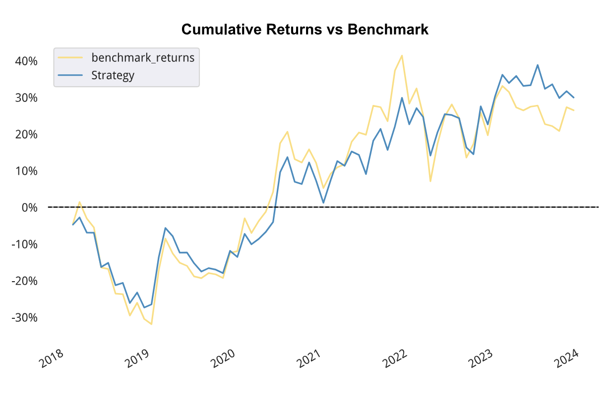 Cumulative Return Comparison
As shown in the chart, during the downturns of 2018, 2022, and 2023, stocks with higher dividend yields proved more resilient. Conversely, during the bull market from 2019 to 2021, high-dividend stocks underperformed other stocks in terms of upside.
info
Research platform users, please double-click `/reports/moonshot_v3.html` to view the detailed report. This directory and file can be found in the Jupyter Lab sidebar.Why do high-dividend stocks underperform during bull markets? Because a significant proportion of these stocks are held by value investors who constantly monitor whether prices have deviated excessively from intrinsic value, making dividend yield an anchoring tool for price. In contrast, speculative "junk" stocks rely on imagination and stories, free from any anchoring constraints.
Similarly, in bear markets, high-dividend stocks are less prone to sharp declines: if prices fall too far below intrinsic value, value investors step in to buy.
However, over the long term, high-dividend stocks yield higher cumulative returns, exhibiting significant alpha and Sharpe ratios, with lower volatility and a better investment experience. The "rose of time" is worth holding.
ParquetUnifiedStorage
ParquetUnifiedStorage is a simple local storage solution. We introduced it in the previous article; this section expands on it to support multiple data access methods and automatic updates.
Its usage involves passing a callback function when defining the store. This callback automatically fetches data from the source if local cache is missing. Thus, callers only need to use store.load_data(start, end) to automatically retrieve data within the [start, end] interval, fully leveraging the cache. This is an excellent tool for small-scale research without dedicated technical team support.
Aside: Pagination in Tushare
Tushare queries generally have a 6,000-record limit. However, some queries allow specifying start_date and end_date parameters. In such cases, the size of the returned dataset is uncertain; if the time span is long, the dataset size may exceed this limit.
In such scenarios, according to the official documentation, we can modify query conditions to reduce the size of the returned dataset, ensuring completeness. For example, to fetch one year of daily data for all China A-shares, we can iterate through the security list or by date. This ensures each returned result set is complete. However, this inevitably incurs performance penalties. For instance, the former involves approximately 5,000 network requests, while the latter involves about 250 requests. Based on the maximum dataset rows per request, theoretically, only about 225 requests are needed. Thus, there is still at least a 10% optimization space.
tip
The number of China A-shares has expanded to the current 5,413 in recent years. Before 2018, the total number of listed companies was around 1,800. Therefore, when iterating through years prior to 2018, each request utilizes less than one-third of the return capacity, resulting in greater performance waste.In the screenshot below, the left image shows the documentation for the daily API for fetching daily market data. Here, we see it does not support pagination queries. However, if we navigate to the Data Tools page, we can see that this API does support pagination.
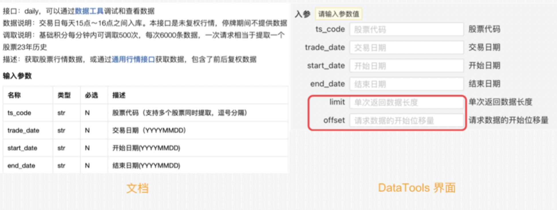
As shown in the image, the two parameters used for pagination are offset and limit. However, there is a hidden issue: offset itself has a maximum limit, such as 100,000. This adds complexity to the algorithm: we must consider cases where, for a single [start, end] query, the theoretical result count is 150,000 records, but only 100,000 can be returned. Therefore, we must re-query, but we don’t know on which day the 100,000 records are truncated. We must also determine two things:
- The time order of Tushare query returns.
- How to determine the truncation date.
The following code is valid only for this API. When applying this to other data, we must consider the time order of Tushare’s return results, which affects the determination of the next query interval.
# example-2
def _fetch_dv_ttm(start: datetime.date, end: datetime.date):
"""Recursively fetch complete daily_basic data, handling offset limit issues"""
dfs = []
pro = ts.pro_api()
cols = "ts_code,trade_date,dv_ttm,total_mv,turnover_rate,pe_ttm"
page_size = 6_000
offset_limit = 100_000
current_start = start
current_end = end
def fetch_batch(batch_start: datetime.date, batch_end: datetime.date):
batch_dfs = []
last_trade_date = None
for i in range(0, int(offset_limit / page_size)):
offset = i * page_size
df = pro.daily_basic(
start_date=batch_start.strftime("%Y%m%d"),
end_date=batch_end.strftime("%Y%m%d"),
fields=cols,
offset=offset,
pagesize=page_size,
)
if len(df) == 0:
break
batch_dfs.append(df)
last_trade_date = df.iloc[-1]["trade_date"] # Date of the last record
# If returned data is less than page_size, fetching is complete
if len(df) < page_size:
return batch_dfs, None
# If offset_limit is reached, return the last fetched trade date
return batch_dfs, last_trade_date
# Main loop: handle cases requiring multiple calls
while current_start <= current_end:
batch_dfs, last_date = fetch_batch(current_start, current_end)
print(f"Fetching data: {current_start} ~ {current_end}, last data date: {last_date}")
dfs.extend(batch_dfs)
if last_date is None:
# Data fetching complete
break
# Convert last_date to datetime.date format
last_date_obj = datetime.datetime.strptime(last_date, "%Y%m%d").date()
# Ensure new_end is not less than start
if last_date_obj < start:
break
current_end = last_date_obj
if dfs:
result_df = pd.concat(dfs, ignore_index=True)
# Deduplicate, as there may be duplicate date data
result_df = result_df.drop_duplicates(subset=["ts_code", "trade_date"])
# Sort by trade date
result_df = result_df.sort_values(["trade_date", "ts_code"])
return result_df
else:
return pd.DataFrame()In the same start-end interval (October 8, 2019, to December 31, 2019), Example 1 takes 45.5 seconds; Example 2 takes about 24 seconds. If we fetch data from an earlier period, this acceleration ratio would be even greater, as there were fewer listed companies in earlier years.
Nevertheless, we must still use these parameters cautiously. At a minimum, prepare regression tests to detect changes immediately if Tushare modifies its API.