Reproducing Research: Screening for Consecutive 2-Year Dividends
This series has been running for quite some time. Before we begin, let’s set the context. For this installment, we are reproducing a CICC research report from December 2023 titled "A Bird in the Hand: A Preferred Dividend Strategy." It is a fundamental strategy. By implementing this report, we aim to learn:
abstract
1. How to acquire various fundamental data, along with explanations of their meanings and compilation methods. 2. How to implement a monthly rebalancing backtest strategy. 3. How to obtain a basic dividend-preferred strategy that can be adapted for live trading by adjusting parameters.- Market data. Essential for any strategy, at least for calculating forward returns.
- Dividend yield. Used to screen stocks by dividend yield and to calculate the two-year average dividend yield factor.
- Dividend records. Only companies that have paid dividends for the past two consecutive years are eligible.
- Audit opinions. Only companies without qualified audit opinions in the past ten years are eligible.
- Market cap data. Only companies with a market capitalization greater than 5 billion RMB are eligible.
- Net profit, operating revenue, and operating profit data. Used to calculate the net profit stability factor.
- Changes in shareholder count.
- Turnover rate. Used to calculate turnover volatility.
- PE (TTM). Used to calculate the EP factor.
- Operating cash flow data. Used to calculate the operating cash flow-to-assets ratio factor.
- Total assets data. Together with item 10, used to calculate the operating cash flow-to-assets ratio factor.
- Surplus reserve data. Together with item 11, used to calculate the retained earnings-to-assets ratio factor.
import tushare as ts
from helper import qfq_adjustment
from fetchers import fetch_bars_ext, fetch_dv_ttm
from store import ParquetUnifiedStorage, CalendarModel
from moonshot import MoonshotIn previous parts of this series, we acquired the data for steps 1–2 and implemented stock pool screening based on dividend yield. The backtest results show that using only the dividend yield factor can generate certain annualized excess returns and a better Sharpe ratio.
In this installment, we will explore how to incorporate dividend data. The research report requires that only companies with dividends paid for the past two consecutive years be included in the stock pool. This is a seemingly simple but technically complex requirement. It involves some "magic" combining multiple pandas techniques to provide a concise implementation for a simple need, which is precisely the goal the author has always pursued.
Acquiring Dividend Data
In the previous article, we acquired dividend yield data. However, to implement the "consecutive two-year dividend" condition precisely, we cannot simply treat "consecutive two-year dividend yield > 0" as "consecutive two-year dividends." Instead, we must directly acquire the raw dividend records.
info
The dividend yield obtained via `daily_basic` is a rolling 12-month dividend yield. Based on its calculation method, a scenario may arise where a company pays a dividend in December 2023 but none in 2024. Yet, until November 2024, the dividend yield will remain positive. Consequently, in February 2025, when we ask if the stock has paid dividends for two consecutive years, we might get an incorrect result. In this regard, dividend records are slightly more precise.The interface signature is as follows:
def dividend(ts_code: str|None = None,
ann_date: str|None = None,
record_date: str|None = None,
ex_date: str|None = None,
imp_ann_date: str|None = None):
passHowever, if we query using these "listed" parameters, the data volume returned per query is small, leading to excessively long acquisition times. Here, we discover a hidden parameter, end_date. You can decide whether to use it based on your specific situation. Let’s compare the number of records obtained using various parameters:
pro = ts.pro_api()
df_ann = pro.dividend(ann_date="20250419")
print("ann_date 一次返回数据:", len(df_ann))
df_end = pro.dividend(end_date="20241231", offse=0, limit=6000)
print("end_date 一次返回数据:", len(df_end))
df_ex = pro.dividend(ex_date="20250419")
print("ex_date 一次返回数据:", len(df_ex))
df_record = pro.dividend(record_date="20250419")
print("record_date 一次返回数据:", len(df_record))
df_imp = pro.dividend(imp_ann_date="20250419")
print("imp_ann_date 一次返回数据:", len(df_imp))As shown, using the end_date parameter yields significantly more data than other parameters; however, its limit is not the common 6000 but restricted to 2000. We must note these behavioral inconsistencies.
Since the limit is only 2000, and there are over 5,000 stocks in China A-shares, we must call the API multiple times using offset/limit to acquire all data for a single day when using end_date.
The following code demonstrates how to acquire data within the interval [start, end]:
def fetch_dividend(start: datetime.date, end: datetime.date):
"""每年分红除权情况
Args:
start (datetime.date): 起始日期
end (datetime.date): 截止日期
Returns:
返回 dataframe, date 为公告日期,fiscal_year 为公告对应财年
"""
dfs = []
limit = 2000
pro = ts.pro_api()
for yr in range(start.year, end.year + 1):
dt = f"{yr}1231"
# 对每一个交易日,都可能有超过 limit 条记录
for offset in range(0, 99):
df = pro.dividend(end_date=dt, offset=offset * limit, limit=limit)
dfs.append(df)
if len(df) < 2000:
break
# 如果取太快,会导致 tushare 拒绝访问
data = pd.concat(dfs)
data["date"] = pd.to_datetime(data["ann_date"]).dt.date
data["fiscal_year"] = pd.to_datetime(data["end_date"]).dt.year
return (
data.rename(columns={"ts_code": "asset"})
.drop(["end_date", "ann_date"], axis=1)
.dropna(subset=["date"])
)attention
In earlier chapters of this series, when calculating the date list between `[start, end]`, we generally used `bdate_range`. This retrieves a list of dates excluding Saturdays and Sundays (though it doesn’t account for Golden Week holidays). Using it for trading data is fine. However, fundamental data may be published on any day, so here we must iterate through the entire calendar to ensure no data is missed. Have you ever made a similar mistake, wasting a weekend debugging?Now, we use the cache we previously developed to store this data:
# 本段代码已在课程环境中运行,数据已缓存,请勿重复运行
path = data_home / "rw/dividend.parquet"
store = ParquetUnifiedStorage(path, calendar)
for yr in (2018, 2019, 2020, 2021, 2022, 2023):
start = datetime.date(yr, 1, 1)
end = datetime.date(yr, 12, 31)
data = fetch_dividend(start, end)
store.append_data(data[data["div_proc"] == "实施"])
print(store.start, store.end)
storepath = data_home / "rw/dividend.parquet"
store = ParquetUnifiedStorage(path, calendar)
for yr in (2018, 2019, 2020, 2021, 2022, 2023):
start = datetime.date(yr, 1, 1)
end = datetime.date(yr, 12, 31)
data = fetch_dividend(start, end)
store.append_data(data[data["div_proc"] == "实施"])
print(store.start, store.end)
store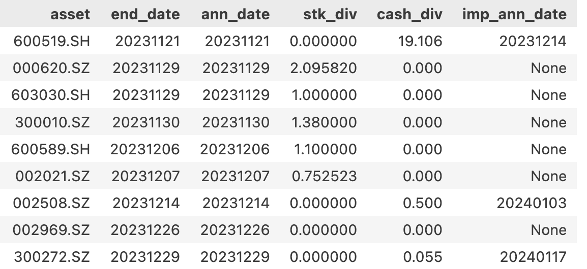 Raw Dividend Records
We fetch data in segments to ensure that if an error occurs, we do not lose too much data.
The documentation does not explain how these records are compiled. Based on our analysis, a company may pay dividends multiple times within a year (unfortunately, such companies are rare, forcing you to abandon value investing and switch to quantitative trading!). For each dividend payment, there may be multiple records corresponding to the proposal, shareholder meeting approval, and implementation stages.
For our current requirement, we only need to focus on the "proposal" stage. Once a proposal is released, speculative capital moves in immediately, without waiting for the implementation stage. Within the proposal, we only need to focus on end_date and ann_date, which are key to calculating whether there have been dividends for two consecutive years.
However, please note that in the example code, we save records where div_proc equals "implementation". This record contains all information from the proposal stage and provides additional information from the implementation stage, which can be useful for other purposes in the future. However, we must be careful: during backtesting, when we treat ann_date as the latest moment, we cannot read cash_div, record_date, or ex_date information, as they would constitute "future data."
tip
Tushare’s records provide after-tax dividends (`cash_div`), but the documentation does not explicitly state its calculation method. Discussion is welcome! According to relevant regulations, corporate and individual shareholders have different dividend tax rates, and individual shareholders’ tax rates vary based on holding periods. Therefore, theoretically, each `cash_div_tax` should correspond to multiple `cash_div` values—depending on who is reading it.Preprocessing and Index Generation
The key to determining "whether dividends were paid for two consecutive years" is to check, at the end of each month, whether the dividend plans for the previous two fiscal years (or this year and last year) have been announced. If so, we mark that month as "satisfying the consecutive dividend condition" (True); otherwise, False.
Therefore, we only need to care about the asset, end_date, and ann_date columns in the data. To facilitate comparison and lookup, we should convert the latter two into fiscal_year (integer, corresponding fiscal year) and announce_ym (year-month of dividend announcement).
Thus, we must first perform the following conversions:
def pre_process(
store, start: datetime.date | None = None, end: datetime.date | None = None
):
df = store.get_and_fetch(start or store.start, end or store.end, call_direct=True)
df["month"] = pd.to_datetime(df["date"]).dt.to_period("M")
# 某些个股在一个财年,可能会有多次分红,我们取最早的一次
(
df.sort_values(["asset", "fiscal_year", "date"])
.groupby(["asset", "fiscal_year"], as_index=False)
.first()
)
cols = ["asset", "month", "fiscal_year"]
return df[cols].set_index(["asset", "month"])
calendar = CalendarModel(data_home / "rw/calendar.parquet")
path = data_home / "rw/dividend.parquet"
store = ParquetUnifiedStorage(path, calendar, fetch_data_func=fetch_dividend)
start = datetime.date(2018, 10, 30)
end = datetime.date(2023, 11, 30)
df = pre_process(store, start, end)
display(df.head())
df.query("asset == '000001.SZ'")The core idea of preprocessing is to convert fine-grained time data into coarse-grained time data. This is one of the core techniques in monthly backtesting. After such conversion, data lookup, alignment, and offset calculations become effortless.
Other notable points include that some stocks may pay dividends multiple times within a fiscal year. In such cases, we need to deduplicate, keeping only the earliest dividend information, as the earliest record is sufficient to indicate that dividends were paid in that fiscal year.
At the end of this example, we extract a small segment of records for PAYH. From this record, we can infer that from March 2022 until the end of that year, we can consider PAYH to have satisfied the "consecutive two-year dividend" condition for 2020 and 2021. However, from January to February 2022, the past two fiscal years are 2020 and 2021. While 2021 might still pay dividends, the financial report may not yet have been disclosed. In this case, should we consider PAYH to satisfy the "consecutive two-year dividend" condition or not? To be or not to be, that is indeed the question. The research report does not provide an answer.
Here, we only consider the majority case: if there are no dividend records before April of the current year, and dividends were paid in the previous two years, we still count it as "consecutive two-year dividends." However, there are exceptions. Good companies release annual report forecasts early; if the annual report is released only in April, it is likely that there will be no dividend—this is equivalent to saying that if the third-to-last and second-to-last years had good operating performance, but the last year’s performance deteriorated, we must wait until the end of April to confirm this. This introduces some unfavorable factors into our strategy.
Code Implementation for Consecutive Two-Year Dividends
We have just preprocessed the data and clarified what "consecutive two-year dividends" means at specific time nodes.
Now, how do we code this logic?
First, let’s clarify our goal: to obtain an output where, for every asset and every month, there is a flag indicating whether that asset satisfies the "consecutive two-year dividend" condition in that month.
Let’s look at what this result table should look like:
all_assets = df.index.levels[0].unique()
months = df.index.levels[1].unique()
all_months = pd.period_range(start=months.min(), end=months.max(), freq="M")
# 生成所有可能的(月份,股票)组合作为基础索引
index = pd.MultiIndex.from_product([all_assets, all_months], names=["asset", "month"])
# result_df 目前是一个空表格
result_df = pd.DataFrame(columns=["consective_div"], index=index)
result_df.tail()Next, we expand the table regarding fiscal_year and announce_ym obtained earlier to align with the above result_df. After alignment, the remaining calculations become as simple as mapping from one table to another.
# 按结果表格进行索引展开
expanded = pd.merge(pd.DataFrame(index=index),
df, how="left",
left_index=True,
right_index=True
)
# 将 fiscal_year 前向填充
expanded = expanded.groupby(level = "asset").ffill()
expanded.tail()Now, we only need to groupby asset on the expanded dataframe above, enable a sliding window of size 24 in each group, and check if the index month is within the fiscal_year set of the sliding window.
# example-consective-div
def calc_asset_flag(group: pd.DataFrame):
df = group.droplevel(level=0)
df["month_num"] = df.index.month
df["year"] = df.index.year
# 这里无法使用 rolling,因为 rolling 后面要跟聚合函数,不能返回 set
df["prev_fiscal_set"] = [
set(x) for x in df["fiscal_year"].rolling(24)
]
def calc_row_flag(row):
prev_fiscal = row["prev_fiscal_set"]
month_num = row["month_num"]
year = row["year"]
if month_num > 4: # 4 月之后,必须最近两年财年都有分红
flag = ((year - 1) in prev_fiscal) and ((year - 2) in prev_fiscal)
return flag
else: # 4 月之前,最近两财年有分红,或者之前两个财年有分红。
flag = (((year - 1) in prev_fiscal) and ((year - 2) in prev_fiscal)) or (
((year - 2) in prev_fiscal) and ((year - 3) in prev_fiscal)
)
return flag
df["consective_div"] = df.apply(calc_row_flag, axis=1)
return df.drop(columns=["month_num", "year", "prev_fiscal_set"])
consective_div = expanded.groupby(level="asset").apply(calc_asset_flag)
consective_div.tail()
There are two notable points in this code. First, when mentioning "rolling" evaluation, we easily think of using sliding windows. However, at line 7, we use a loop instead of rolling.apply to find the values from the previous two years for the corresponding row. This is because rolling.apply is generally applied to aggregation operations, and the function’s return value must be numeric.
The second point is line 29, which is essentially still a loop. Considering that calc_row_flag only performs within-row comparisons, this can be further optimized to enable parallel processing. On my computer, this code runs in 13 seconds, which is still a bit slow.
How do we verify the correctness of this logic? For PAYH, we see that from March 2020 onwards, the flag for each month is 1; this is correct because it pays dividends every year. We also found a counterexample, 920819, which has the following dividend records:
df_ = ts.pro_api().dividend(ts_code = "920819.BJ")
df_[df_.div_proc == '实施'][["ts_code", "end_date", "ann_date"]]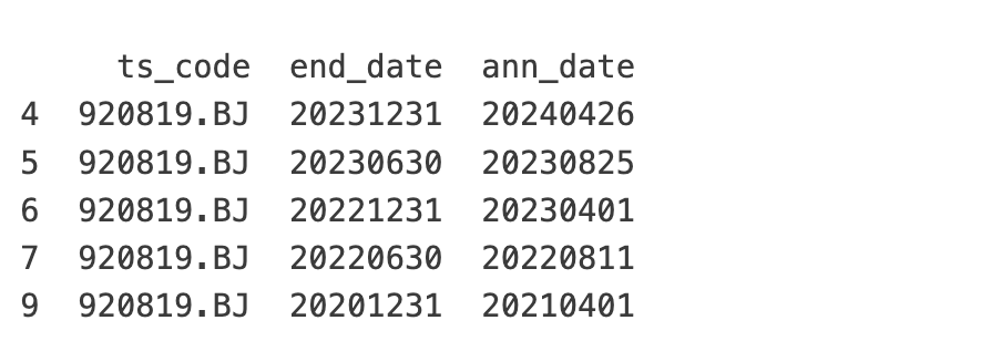
It paid dividends in 2020, 2022, and 2024, but not in 2021 (there was a proposal, but it was not approved). Therefore, only from January 2024 onwards does the "consecutive two-year dividend" query show that it satisfies the condition.
This proves that our implementation is correct.
Applying Dividend Screening
from IPython.display import clear_output
def dividend_yield_screen(data: pd.DataFrame, n: int = 500) -> pd.Series:
"""股息率筛选方法
对每个月的股息率进行排名,选择前n名股票,标记为1,
与现有flag进行逻辑与运算
Args:
n: 每月选择的股票数量,默认500
"""
logger.info("开始进行股息率筛选...")
if "dv_ttm" not in data.columns:
raise ValueError("数据中不存在 dv_ttm 列,无法应用筛选器")
def rank_top_n(group):
# 计算每个股票在当月的排名(降序,股息率高的排名靠前)
ranks = group.rank(method="first", ascending=False)
return (ranks <= n).astype(int)
# 按date分组,对 dividend_rate_ttm 进行排名筛选
dividend_flags = data.groupby(level="month")["dv_ttm"].transform(rank_top_n)
logger.info(f"已筛选出前{n}名股息率股")
return dividend_flags
def consective_dividend_screen(data):
return data.consective_div
start = datetime.date(2018, 1, 1)
end = datetime.date(2023, 12, 31)
store_path = data_home / "rw/bars.parquet"
bars_store = ParquetUnifiedStorage(store_path, calendar, fetch_data_func=fetch_bars_ext)
barss = bars_store.get_and_fetch(start, end)
ms = Moonshot(barss)
# consecative_div 示例 example-consective-div
ms.append_factor(consective_div, "consective_div")
# 我们把上一篇的股息率筛选也加上
store_path = data_home / "rw/dv_ttm.parquet"
dv_store = ParquetUnifiedStorage(store_path, calendar, fetch_data_func=fetch_dv_ttm)
dv_ttm = dv_store.get_and_fetch(start, end)
ms.append_factor(dv_ttm, "dv_ttm", resample_method="last")
output = get_jupyter_root_dir() / "reports/moonshot_v4.html"
# 筛选! 回测! 报告!
(
ms.screen(dividend_yield_screen, data=ms.data, n=500)
.screen(consective_dividend_screen, data=ms.data)
.calculate_returns(True)
.report(kind="html", output=output, periods_per_year=12)
)
clear_output()Finally, we obtain the following report:
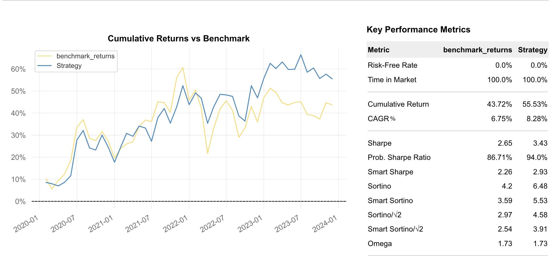
info
Research platform users, please double-click `/reports/moonshot_v4.html` to view the more detailed report. This directory and file can be found in the sidebar of Jupyter Lab.If you are interested in the code in this article, you can become a member. We provide data, code, and a running environment to immediately run and verify strategies. If you are not familiar with the technical details in the article, you can take our courses.