
Moonshot Is All You Need: Finalizing a High-Sharpe Dividend Strategy
We have covered the Moonshot framework and dividend strategy implementation across four parts. This is the final installment of the series. Using the previously established Moonshot backtest framework, we will finally complete the construction of the dividend strategy.
Factor Construction Methodology
The core of a dividend strategy is the dividend yield. In fact, the dividend yield factor is one of the earliest asset pricing factors. In a series of classic papers, including Harvey, Liu & Zhu (2016), Dividend Yield is an important component of valuation factors, but its significance is generally weaker than other classic factors such as market cap and P/M. Dividend yield often appears in companies with stable cash flows, representing one side of the value factor. Furthermore, dividend income, capital gains, and risk aversion can be appropriately explained from an economic perspective, as can management signaling theory.
Research reports have constructed multiple factors from the perspectives of dividend income, capital gains, and risk avoidance, which have certain predictive effects on a stock's future dividends. Below, we briefly describe the factor construction methods; the specific code for factor construction is provided later in the text.
Top 500 Dividend Yield (DP) and 2-Year Average Dividend Yield Standard Score (DP2)
Meaning: Stocks with high dividends tend to have high future dividend yields and per-share dividends.
Calculation: The calculation of dividend yield was demonstrated in the aforementioned series. We retrieve the dv_ttm field from the Tushare daily_basic interface. The 2-year average dividend yield, dividend_yield_2y_avg, is calculated by combining the dv_ttm and close prices from one year ago with the current dv_ttm and close. See the code for specific calculation details.
Payout Ratio (DPR)
Meaning: Stocks with high payout ratios may struggle to sustain future dividends, while moderate payout ratios may favor future returns. Specifically, if the payout ratio is low, it may indicate poor dividend performance, leading to average portfolio returns; if the payout ratio is high, dividend behavior may be unsustainable.
Calculation: The payout ratio is dividends/net profit, which means Payout Ratio = Dividend Yield / EP = Dividend Yield * PE. Therefore, we retrieve pe_ttm * dv_ttm from the daily_basic interface.
Market Cap Screening (Total Market Cap > 5 Billion RMB)
Meaning: Small market caps exacerbate the overall volatility of the portfolio.
Calculation: Retrieve total_mv from the Tushare daily_basic interface, in units of 10,000 RMB.
Turnover Volatility
Meaning: Turnover volatility has good stock selection capability in the dividend stock pool. Introducing a low-volatility factor based on turnover volatility helps improve the portfolio's margin of safety.
Calculation: Calculate the standard deviation over the past month using turnover_rate_f (free float turnover rate) from the Tushare daily_basic interface.
EP Standard Score
Meaning: Mean reversion of valuation grouped by EP is significant, with the maximum portfolio having the lowest valuation.
Calculation: In the daily_basic interface, you can directly use PE to reverse-calculate EP, then take the 5-year standard score.
TTM Growth of Dividend Amount Compared to Previous Month
Meaning: Continuous, stable, and growing dividends convey management's confidence in cash flow and profit quality, benefiting long-term shareholder returns and valuation stability.
Calculation: Calculate dividend_ttm using dv_ttm and total market cap, then compare monthly changes.
Shareholder Count Standard Score
Meaning: A decrease in shareholder count may indicate that investors with information advantages are accumulating shares, anticipating future company performance.
Calculation: Calculate historical sequences via the stk_holdernumber interface.
Audit Opinion (Exclude Non-Standard Unqualified)
Meaning: Non-standard audit opinions often signal increased financial uncertainty or potential risk events.
Calculation and Scope: Read audit_result via the fina_audit interface.
Operating Cash Flow to Total Assets Ratio
Meaning: If a company has ample cash flow, it helps maintain high future dividend levels. However, if a company with tight cash or cash flow still chooses cash dividends, this behavior may be unsustainable and carries certain risks.
Calculation: Retrieve n_cashflow_act from cashflow_vip, and total_assets from balancesheet_vip, then calculate n_cashflow_act / total_assets.
Retained Earnings to Total Assets Ratio
Meaning: Using the retained earnings to total assets ratio to measure lifecycle, mature companies have a higher proportion of retained earnings to total assets, where dividend payments are concentrated.
Calculation: Retrieve undistr_porfit and total_assets fields from balancesheet_vip, and calculate RETA = undistr_porfit / total_assets.
Net Profit Performance Stability (np_std)
Meaning: When the current financial stability factor (e.g., standard score of net profit over the past eight periods) is large, the future ROE of dividend stocks may maintain high levels. Therefore, the financial stability factor has certain predictive power for a company's future profitability.
Calculation: Retrieve n_income_attr_p from the income_vip interface and calculate the standard score of net profit over the past eight periods.
Data Preparation
The code for this section is too extensive to display in full. On the Kuangti Research Platform, we provide complete, runnable code. If readers are interested in strategy verification, they can apply for membership to access it.
Backtest
Our backtest period is set from November 30, 2018, to November 30, 2023. In fact, due to the "New Nine Guidelines" (Guo Jiu Tiao), the strategy's performance in the subsequent period would be even better, which we will introduce in future articles.
Since this strategy uses too many data varieties and the data cleaning process is complex, it is best to have a robust data acquisition framework to support backtesting across different time intervals. In this article, we will not expand further on this.
Following the logic of the Moonshot backtest framework, we first need to acquire market data and construct a Moonshot instance:
import sys
sys.path.append(str(Path(".").parent))
import tushare as ts
from helper import qfq_adjustment
from fetchers import fetch_bars
from store import ParquetUnifiedStorage, CalendarModel
from moonshot import Moonshot
# get candles data
start = datetime.date(2018, 11, 30)
end = datetime.date(2023, 11, 30)
calendar= CalendarModel(data_home/"rw/calendar.parquet")
store_path = data_home / "rw/bars.parquet"
bars_store = ParquetUnifiedStorage(store_path, calendar, fetch_data_func=fetch_bars)
barss = bars_store.get_and_fetch(start, end)
barss = qfq_adjustment(barss, "adj_factor")
barss.tail()This part of the code is simple and omitted. Please obtain the complete code from the Planet.
Next, we instantiate Moonshot and add factors:
ms = Moonshot(barss)
# ADD FACTORS
daily_basic_after = pd.read_parquet(data_home / "rw/moonshot/daily_after.parquet")
ms.append_factor(
daily_basic_after, "total_mv", resample_method="last"
)
ms.append_factor(
daily_basic_after, "dv_ttm", resample_method="last"
)
ms.append_factor(
daily_basic_after,
"dividend_yield_2y_avg",
resample_method="last",
)
ms.append_factor(
daily_basic_after,
"dividend_yield_2y_avg_noffill",
resample_method="last",
)
ms.append_factor(
daily_basic_after, "DPR", resample_method="last"
)
ms.append_factor(
daily_basic_after,
"turnover_rate_f_std",
resample_method="last",
)
ms.append_factor(
daily_basic_after,
"inv_pe_ttm_zscore_5y",
resample_method="last",
)
ms.append_factor(
daily_basic_after,
"dividend_ttm_increase_1M",
resample_method="last",
)
# ADD HOLDERS
holder = pd.read_parquet(data_home / "rw/moonshot/holder_zscore_4y.parquet")
holder.rename(columns={"ts_code": "asset"}, inplace=True)
ms.append_factor(holder, "holder_z_score", resample_method="last")
# ADD AUDIT
final_audit_df = pd.read_parquet(data_home / "rw/moonshot/audit_reserve.parquet")
final_audit_df.rename(columns={"ts_code": "asset"}, inplace=True)
ms.append_factor(final_audit_df, "has_audit_reserve", resample_method="last")
# ADD CASHFLOW, INCOME, BALANCE SHEET
n_cashflow_act = pd.read_parquet(data_home / "rw/moonshot/n_cashflow_act.parquet")
ms.append_factor(n_cashflow_act, "n_cashflow_act", resample_method="last")
income_8q_zscore = pd.read_parquet(data_home / "rw/moonshot/income_8q_zscore.parquet")
income_8q_zscore.rename(columns={"ts_code": "asset"}, inplace=True)
ms.append_factor(income_8q_zscore, "profit_z_score", resample_method="last")
balancesheet_asset_profit = pd.read_parquet(
data_home / "rw/moonshot/assets_undistr_profit.parquet"
)
ms.append_factor(balancesheet_asset_profit, "undistr_porfit", resample_method="last")
ms.append_factor(balancesheet_asset_profit, "total_assets", resample_method="last")
During the above process, null values may be introduced or already exist. Before backtesting, we must also perform data filling:
ms.data.sort_index(level=['month', 'asset'], inplace=True)
cols_to_ffill = ['total_mv', 'dv_ttm', 'dividend_yield_2y_avg', 'DPR', 'turnover_rate_f_std',
'inv_pe_ttm_zscore_5y', 'dividend_ttm_increase_1M', 'holder_z_score',
'has_audit_reserve', 'n_cashflow_act', 'profit_z_score',
'undistr_porfit', 'total_assets']
# 在每个 asset 内按时间(month)前向填充
ms.data[cols_to_ffill] = (
ms.data.groupby(level='asset')[cols_to_ffill]
.ffill()
)Next, according to the strategy requirements, we first build the stock pool, which has four conditions:
- Top 500 in dividend yield per period.
- Consecutive two-year dividends. Translated to
dividend_yield_2y_avg_noffill > 0, wheredividend_yield_2y_avg_noffillrefers to the result ofdividend_yield_2y_avgcalculation without null value filling. If a stock is empty, 0, or negative on this factor, it obviously does not have consecutive 2-year dividends. - No audit opinions in the past ten years.
- Market cap greater than 5 billion RMB.
def stock_pool_filter(data: pd.DataFrame) -> pd.Series:
df = data.copy()
# 股息率前 500 名
dv_rank = df.groupby(level="month")['dv_ttm'].transform(lambda x: x.rank(method='first', ascending=False))
cond1 = dv_rank <= 500
cond2 = df['dividend_yield_2y_avg_noffill'] > 0 # 连续两年有分红
cond3 = df['has_audit_reserve'] == False # 无审计保留意见
cond4 = df['total_mv'] >= 500000 # 总市值 > 50亿,总市值单位是 (万元)
flag = cond1 & cond2 & cond3 & cond4
return flag.astype(int)The function factor_screen describes the core stock selection factors. According to the research report's understanding, for indicators that are significantly effective in the dividend stock pool, we will use the standard scores of the indicators; for stocks with lower effectiveness, we will construct threshold signals to describe relevant information.
Specifically, this includes 4 standard scores and 6 signal events:
Two-year average dividend yield
dividend_yield_2y_avg: The larger, the better.Net profit performance stability
profit_z_score: The larger, the better.Shareholder count change
holder_z_score: The smaller, the better.Turnover volatility
turnover_rate_f_std: The smaller, the better.Payout ratio top 1/5 +1, Payout ratio bottom 1/5 -1, DPR
Operating cash flow to total assets ratio bottom 1/5 -1,
n_cashflow_act / total_assetsRetained earnings to assets ratio bottom 1/5 -1,
undistr_porfit / total_assetsEP top 1/5 stocks +1, EP bottom 1/5 stocks -1,
inv_pe_ttm_zscore_5yBetween dividend proposal date and shareholders' meeting announcement date: Skipped due to lack of data.
Recent 1-month dividend TTM growth +1,
dividend_ttm_increase_1M
We encapsulate this process into a function:
def factor_screen(data: pd.DataFrame, top_n: int = 30) -> pd.Series:
df = data.copy()
# 只对上一层筛选通过的股票打分
if 'flag' in df.columns:
df = df[df['flag'] == 1].copy()
factor_rank_info = {
'dividend_yield_2y_avg': True,
'profit_z_score': True,
'holder_z_score': False, # 越小越好
'turnover_rate_f_std': False, # 越小越好
}
def zscore_func(s, is_positive):
s = s.copy()
if not is_positive:
s = -s
mean = s.mean(skipna=True)
std = s.std(skipna=True)
if pd.isna(std) or std == 0:
return pd.Series(0, index=s.index)
z = (s - mean) / std
return z.fillna(0)
# 计算财务比率
df['undistr_ratio'] = np.where(df['total_assets'] == 0, np.nan, df['undistr_porfit'] / df['total_assets'])
df['cf_ratio'] = np.where(df['total_assets'] == 0, np.nan, df['n_cashflow_act'] / df['total_assets'])
# 派息率前5分之一+1 派息率后5分之一 -1, DPR
df['score_dpr'] = df.groupby('month')['DPR'].transform(
lambda s: (
(s >= s.quantile(0.8)).astype(int) - # 前 20% → +1
(s <= s.quantile(0.2)).astype(int) # 后 20% → -1
).fillna(0)
)
# EP 前5分之一+1 EP 后5分之一-1 inv_pe_ttm_zscore_5y
df['score_ep'] = df.groupby('month')['inv_pe_ttm_zscore_5y'].transform(
lambda s: ((s >= s.quantile(0.8)).astype(int) - (s <= s.quantile(0.2)).astype(int)).fillna(0)
)
# 经营现金流资产比后5分之一 n_cashflow_act / total_assets -1
df['score_cf'] = df.groupby('month')['cf_ratio'].transform(
lambda s: (-1 * (s <= s.quantile(0.2))).fillna(0).astype(int)
)
# 留存收益/资产比后5分之一 -1 undistr_porfit / total_assets
df['score_undistr'] = df.groupby('month')['undistr_ratio'].transform(
lambda s: (-1 * (s <= s.quantile(0.2))).fillna(0).astype(int)
)
# score_dividend_increase
df['score_dividend_increase'] = df['dividend_ttm_increase_1M'].fillna(False).astype(int)
for fac, is_positive in factor_rank_info.items():
df[f"{fac}_score"] = df.groupby('month')[fac].transform(lambda s: zscore_func(s, is_positive))
# 总分
score_cols = [f"{fac}_score" for fac in factor_rank_info] + [
'score_dpr', 'score_cf', 'score_undistr',
'score_ep', 'score_dividend_increase']
df['total_score'] = df[score_cols].sum(axis=1)
# Top-N flag
flag = df.groupby('month')['total_score'].transform(
lambda s: (s.rank(method='first', ascending=False) <= top_n).astype(int)
)
# 对齐回原索引(未筛选股票置 0)
flag = flag.reindex(data.index).fillna(0).astype(int)
return flagNext, we perform screening and backtesting:
from IPython.display import clear_output
ms.screen(stock_pool_filter, data=ms.data)
ms.screen(factor_screen, data=ms.data, top_n=30)
ms.calculate_returns(True)
# 沪深300
pro = ts.pro_api()
hs300 = pro.index_daily(ts_code='000300.SH',
start_date=start.strftime("%Y%m%d"),
end_date=end.strftime("%Y%m%d"))
hs300.index = pd.to_datetime(hs300["trade_date"])
benchmark = hs300["close"].resample('M').last().pct_change()
output = get_jupyter_root_dir() / "reports/moonshot-5.html"
ms.report("html", benchmark = benchmark, output=output, periods_per_year=12)
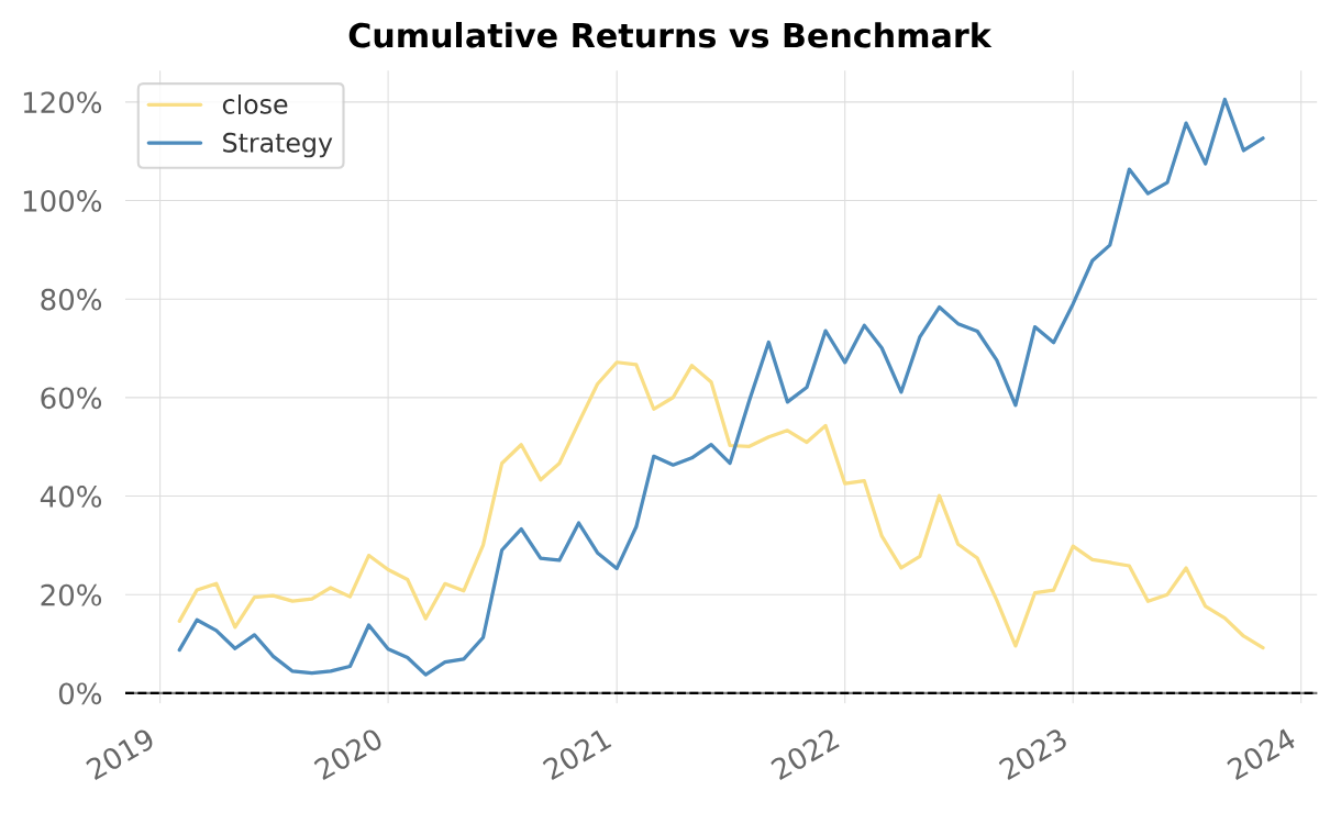
clear_output()You can find strategy.html to view the complete backtest report. Compared to the CSI 300, the dividend strategy shows significant advantages. Here is the comparison chart of their cumulative returns:
Here is a comparison of some important strategy evaluation indicators:
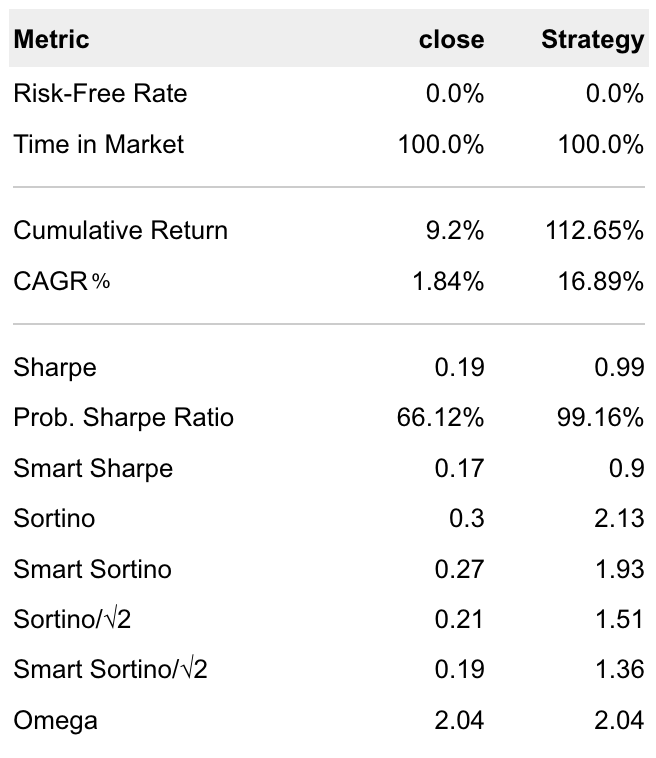
Over the past 5 years, the cumulative return of the dividend strategy is 112.65%, while the CSI 300 is only 9.2%. The annualized return of the dividend strategy reached 16%; meanwhile, the CSI 300 was only 1.84%.
How does this strategy compare to the CSI Dividend Index?
dividend_index = pro.index_daily(ts_code='000922.CSI',
start_date=start.strftime("%Y%m%d"),
end_date=end.strftime("%Y%m%d"))
dividend_index.index = pd.to_datetime(dividend_index["trade_date"])
benchmark = dividend_index["close"].resample('M').last().pct_change()
ms.report("metrics", benchmark = benchmark, periods_per_year=12)As can be seen, this strategy significantly outperforms the CSI Dividend Index across all indicators.