Storing 50TB: PyArrow + Parquet for Tick Data

In the previous note, we argued that HDF5 is more than enough if you only store daily bars and factors. Even querying 40 years of 1-minute bars for a single stock took just 0.2 seconds — plenty fast, as long as you don't need cross-sectional queries at the minute level.

But if you as an individual trader do have the network and hardware for high-frequency trading, handling tick and Level-2 data becomes a must. That pushes you straight into terabyte territory, while you still want millisecond query latency. Or you may genuinely need cross-sectional queries on minute bars. In those cases, HDF5 is no longer up to the job.

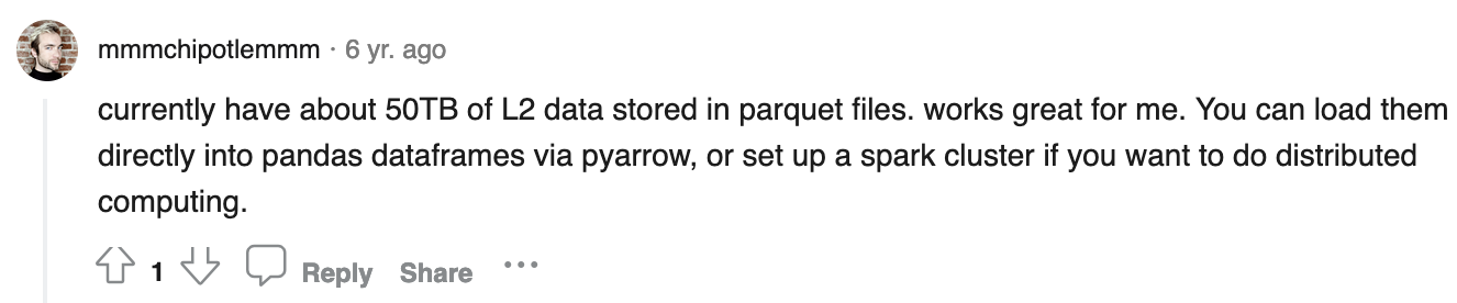
Enter PyArrow + Parquet. They were built for big data in the first place. The “50TB” in the title is not from my own experiment — I don’t have that kind of storage — but the number isn’t made up either:

To introduce PyArrow, we have to start with Apache Arrow. Apache Arrow defines a language-independent, columnar in-memory format for efficient data reads and analytics on CPU/GPU.

PyArrow is the Python implementation of the Apache Arrow library. Apache Arrow also has R, Java, and other implementations. But PyArrow is the first-class citizen — many cutting-edge features land here first, then in R and the rest.

PyArrow supports Python 3.8 to 3.11. Install it with:

1pip install pyarrow

Parquet

Parquet is a data storage format. In big-data storage you’ll also often see Feather. The difference is that Parquet offers RLE compression, dictionary encoding (similar to replacing with category in pandas), and data-page compression. So it is slower than Feather on reads/writes, but much more space-efficient.

Core Concepts

The most basic concepts in PyArrow are:

1. array — a column of homogeneous data, usually allowing None.
2. A set of equal-length array instances forms a Record Batch. A batch can be sliced just like an array.
3. Above batches sits the Table concept. A table consists of columns, each of which is a ChunkedArray.

We’ll also run into the concept of schema, which we’ll explain with examples below.

PyArrow’s main capabilities:

1. Various I/O interfaces (memory and IO interfaces), such as read/write conversion with other common formats like CSV, dataframe, S3, minio, and local files.
2. A tabular datasets view of your data plus related operations.
3. Core compute Functions, such as group-by, aggregations, joins, and queries (expressions, pandas-style).

The English terms in parentheses above match the Arrow documentation directly, so you can look them up when needed.

A Market Data Storage Layout

Although we’re introducing PyArrow + Parquet for Level-2 data, I don’t have a Level-2 data source at hand, so I can’t provide a runnable example for that. Instead, we’ll demonstrate how to write, append, and query data by building a 1-minute bar dataset.

We’ll put all symbols’ 1-minute bars for each day in a single file, with all minute bars under a 1m directory. We’re not using partitioning here, but in practice you’d want to partition minute bars by year. For Level-2 data, you might partition by month or week.

On the other hand, each Parquet file is ideally between 20M and 2GB, so for data at minute frequency and above, consider writing one file per week or at an even coarser granularity.

Here’s an example on-disk layout:

1234567/tmp/pyarrow
├── 1d
├── 1m
│   ├── 2023-12-27.parquet
│   ├── 2023-12-28.parquet
│   └── 2023-12-29.parquet
└── factors

First, define the storage fields:

12345678910111213import pyarrow as pa

schema = pa.schema([
        ("symbol", pa.string()),
        ("frame", pa.date64()),
        ("open", pa.float32()),
        ("high", pa.float32()),
        ("low", pa.float32()),
        ("close", pa.float32()),
        ("volume", pa.float64()),
        ("money", pa.float64()),
        ("factor", pa.float64())
])

PyArrow supports string and date types!

Next, we implement appending and read/write. Since we store each day’s minute bars as one Parquet file, the code is very simple:

12345678910111213141516171819202122import arrow
import pyarrow.parquet as pq

async def save_1m_bars(codes, dt: datetime.datetime):
    tables = None

    for code in codes:
        bars = await Stock.get_bars(code, 240, FrameType.MIN1, end=dt)
        data = [[code] * len(bars)]

        data.extend([
                    bars[key] for key in bars.dtype.names
                ])
        table = pa.Table.from_arrays(data, schema=schema)
        if tables is None:
            tables = table
        else: # 拼接表
            tables = pa.concat_tables([tables, table])

    # 写入磁盘
    name = arrow.get(dt).format("YYYY-MM-DD")
    pq.write_table(tables, f"/tmp/pyarrow/1m/{name}.parquet")

Since we store all stocks and indexes in one big table, we also call concat_tables to stitch them together. In most other similar data structures, whether numpy, pandas, or HDF5, this kind of concatenation is fairly expensive, but in PyArrow it’s almost zero-cost! No data is copied.

Next, let’s show how to call save_1m_bars to save data:

1234codes = ["000001.XSHE", "600000.XSHG"]
for i in (25, 26, 27, 28, 29):
    dt = datetime.datetime(2023, 12, i, 15)
    await save_1m_bars(codes, dt)

Querying Data

Now, let’s read back the data we just wrote:

1234import pyarrow.dataset as ds

dataset = ds.dataset("/tmp/pyarrow/1m")
dataset.files

Here dataset is just metadata. Up to this point, nothing is actually loaded from disk. Loading starts with to_table, or with a query.

The snippet above will list the on-disk files contained in the dataset.

We can convert the dataset into one big table:

12table = dataset.to_table()
table

This will print the table’s field definitions plus a preview of the data.

to_table loads everything into memory. If the dataset is large, you’ll run out of memory. So in many cases you may want to use RecordBatch instead:

12for rb in dataset.to_batches():
    print(rb.to_pandas())

Each RecordBatch has a to_pandas method, which takes you back into familiar territory.

But more often, we’ll load only the slice we need via a query. For that we use the expression syntax in pyarrow.compute, mainly the field function, logical operators, and bitwise operators (not shown here, i.e. & | etc.):

1234import pyarrow.compute as pc

filter = (pc.field("frame") > pc.scalar(datetime.datetime(2023, 12, 28, 15)))
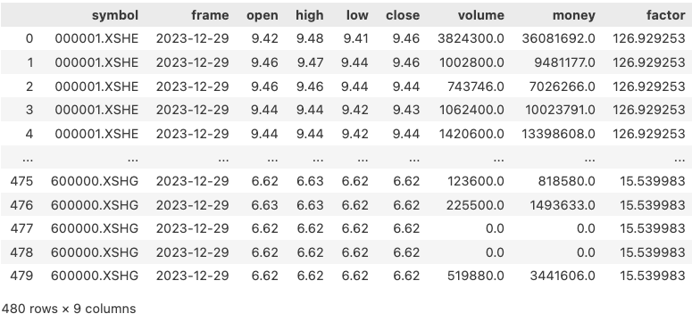
dataset.filter(filter).to_table().to_pandas()

Out of a vast sea of data, we take just one sip. This time we loaded only 480 records into memory.