DeepSeek’s Pit, Not the Grave: Why Junior Devs Can’t Escape

In our Factor Analysis and Machine Learning Strategies course, we provide 18 years of daily data (over 11 million records from 2005 to 2023) for students to conduct factor mining and validation. Initially, we cached this data in memory using the lru_cache decorator from Python’s functools. This approach meant that while the first call took slightly longer (around 5 seconds), subsequent calls were processed in milliseconds.

The Problem

However, this approach created a significant issue: excessive memory consumption. A single factor analysis session could consume over 5GB of RAM. Since JupyterLab lacks the ability to automatically close idle kernels (a feature present in Google Colab and Kaggle), our memory resources were quickly exhausted.

Our data is organized as a dictionary and stored on disk:

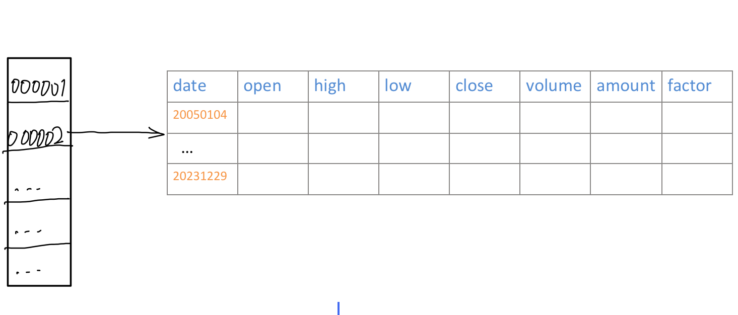
The dictionary keys are stock ticker symbols, and the corresponding values are NumPy structured arrays. This data structure may seem unique, but its rationale will become clear shortly.

Before conducting factor analysis, users load market data by specifying a universe (a stock pool) and a start/end date range. The universe can be a predefined list of securities or simply a target size. The date range allows users to adjust the observation window, which is often done for performance reasons: initially, developers may only need a small subset of data for debugging; once debugging is complete, they run a full backtest or observe data in segments.

The function ultimately returns a DataFrame with a dual index of date and asset (stock ticker), containing columns for OHLC, volume, etc. These columns are adjusted forward based on the end date (a method known as dynamic forward adjustment). Additionally, an amount column is included, which remains unadjusted.

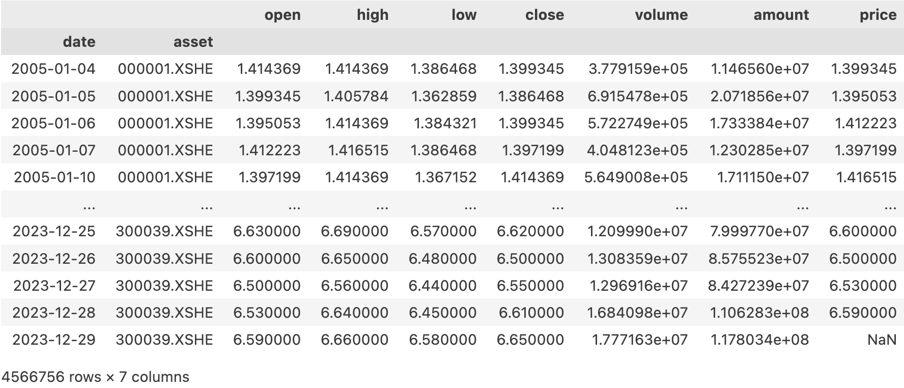
Thus, the function signature is:

1234def load_bars(start_date:datetime.date, 
              end_date:datetime.date, 
              universe: Tuple[str]|int = 500)->pd.DataFrame:
    pass

Students learn by reading our notebook documentation and experimenting with the code cells, potentially modifying and re-running them. This is an interactive process. Generally, a user wait time of under 3 seconds is acceptable. A response time of under 1 second is considered ideal.

Without caching, the initial implementation ran in approximately 5 seconds:

123start = datetime.date(2023, 12,1)
end = datetime.date(2023, 12,31)
%time load_bars(start, end, 2000)

The subsequent tests will use the same parameters.

Of course, using a larger universe would further increase the time.

Since this result exceeds the 3-second threshold, we aimed to optimize the code. Performance optimization is one of the most challenging aspects of programming, as it requires a deep understanding of program execution principles and proficiency across multiple tech stacks. During this process, I explored the capabilities and boundaries of DeepSeek R1, which I hope serves as a useful reference.

The Initial Approach

The initial code was as follows:

1234567891011121314151617181920212223242526272829303132333435363738394041424344454647def load_bars_v1(
    start: datetime.date, end: datetime.date, universe: Tuple[str]|int = 500
)->pd.DataFrame:

    if barss is None:
        with open(os.path.join(data_home, "bars_1d_2005_2023.pkl"), "rb") as f:
            barss = pickle.load(f)

    keys = list(barss.keys())
    if isinstance(universe, int):
        if universe == -1:
            selected_keys = keys
        else:
            selected_keys = random.sample(keys, min(universe, len(keys)))
            try:
                pos = selected_keys.index("000001.XSHE")
                swp = selected_keys[0]
                selected_keys[0] = "000001.XSHE"
                selected_keys[pos] = swp
            except ValueError:
                selected_keys[0] = "000001.XSHE"

    else:
        selected_keys = universe

    dfs = []
    for symbol in selected_keys:
        qry = "frame >= @start & frame <= @end"
        df = pd.DataFrame(barss[symbol]).assign(asset=symbol).query(qry)

        if len(df) == 0:
            logger.debug("no bars for %s from %s to %s", symbol, start, end)
            continue
        # 前复权
        last = df.iloc[-1]["factor"]
        adjust_factor = df["factor"] / last
        adjust = ["open", "high", "low", "close", "volume"]
        df.loc[:, adjust] = df.loc[:, adjust].multiply(adjust_factor, axis="index")

        dfs.append(df)

    df = pd.concat(dfs, ignore_index=True)
    df.set_index(["frame", "asset"], inplace=True)
    df.index.names = ["date", "asset"]
    df.drop("factor", axis=1, inplace=True)
    df["price"] = df["open"].shift(-1)
    return df

The code has been significantly optimized (some suggestions came from AI). For instance, saving data as a dictionary, filtering by universe first, and then concatenating into a DataFrame—rather than saving all data as a DataFrame and filtering via pandas (which would take several times longer)—was a key improvement.

Additionally, during forward adjustment, it used the multiply method to adjust multiple columns in one go, a suggestion provided by AI.

However, the code still contained a for loop. Could eliminating this loop further improve speed?

Below, I attempted to use DeepSeek R1 to address this.

Here is the first round of prompts:

123456789101112131415with open(os.path.join(data_home, "bars_1d_2005_2023.pkl"), "rb") as f:
    data = pickle.load(f)

dfs = []
for symbol, bars in data.items():
    df = pd.DataFrame(bars)
    df["asset"] = symbol
    df = df.rename(columns={"frame": "date"})
    dfs.append(df)

barss = pd.concat(dfs,ignore_index=True).set_index(["date", "asset"]).sort_index()
print(len(barss))

# 定义一个一致的universe，便于比较
universe = barss.index.get_level_values("asset").unique().tolist()

The following code was generated by DeepSeek. We asked it to provide solutions for the most time-consuming parts: filtering and adjustment.

Pandas Implementation

1234567891011121314151617181920212223242526def adjust_pandas(df, selected_symbols, start, end):
    # 筛选数据
    idx = pd.IndexSlice
    filtered = df.loc[idx[start:end, selected_symbols], :]
    
    # 按 asset 分组计算最后复权因子
    grouped = filtered.groupby('asset', group_keys=False)
    last_factor = grouped['factor'].transform('last')
    
    # 计算调整比例
    ratio = filtered['factor'] / last_factor
    
    # 计算复权后字段
    adjusted = filtered.assign(
        open   = filtered['open'] * ratio,
        high   = filtered['high'] * ratio,
        low    = filtered['low'] * ratio,
        close  = filtered['close'] * ratio,
        volume = filtered['volume'] * (last_factor / filtered['factor'])
    )
    
    # 选择最终列并保持索引
    return adjusted[['open', 'high', 'low', 'close', 'volume', 'amount']]

%time adjust_pandas(barss, universe, start, end)
adjust_pandas(barss, universe, start, end)

Although I am familiar with Pandas, there are still some APIs I didn’t know, such as transform. However, using the correct API is precisely the key to boosting performance in Python.

The average runtime for this version was 7 seconds, indicating that Pandas filtering is indeed slow.

We will skip the PyArrow version. The PyArrow version ran in approximately 3.7 seconds, offering only marginal improvement over the original version. This also highlights that in Python 3.11, for loops run quite fast.

Polars Implementation

Here is the Polars version provided by DeepSeek:

123456789101112131415161718192021222324252627import polars as pl

def adjust_polars(df, selected_symbols, start, end):
    # 筛选数据
    filtered = df.filter(
        (pl.col("date").is_between(start, end)) &
        (pl.col("asset").is_in(selected_symbols))
    )
    
    # 计算最后复权因子和调整比例
    adjusted = filtered.with_columns(
        last_factor = pl.col("factor").last().over("asset")
    ).with_columns(
        ratio = pl.col("factor") / pl.col("last_factor"),
        volume_ratio = pl.col("last_factor") / pl.col("factor")
    ).with_columns(
        open   = pl.col("open") * pl.col("ratio"),
        high   = pl.col("high") * pl.col("ratio"),
        low    = pl.col("low") * pl.col("ratio"),
        close  = pl.col("close") * pl.col("ratio"),
        volume = pl.col("volume") * pl.col("volume_ratio")
    )
    
    # 选择最终列
    return adjusted.select(["date", "asset", "open", "high", "low", "close", "volume", "amount"])

adjust_polars(barss, universe, start, end)

I was previously unfamiliar with Polars, and DeepSeek instantly expanded my capabilities. If I had tried to learn this feature through self-study, I am unsure how long it would have taken me to discover the .over API, as this is a unique window operation API in Polars. I couldn’t simply transfer my knowledge from Pandas to it.

However, this version contained an error: it did not adhere to my specified data format, treating barss as a Polars DataFrame with asset and date columns. Using Tongyi Lingma, I corrected this error. The corrected code is as follows:

1%time adjust_polars(pl.from_pandas(barss.reset_index()), universe, start, end)

The resulting runtime was 1.01 seconds, which is very close to our ideal speed.

DuckDB Implementation

Now, let’s look at the DuckDB version it provided:

1234567891011121314151617181920212223242526272829import duckdb

def adjust_duckdb(df, selected_symbols, start, end):
    query = f"""
    SELECT 
        date, asset,
        open * (factor / last_factor) AS open,
        high * (factor / last_factor) AS high,
        low * (factor / last_factor) AS low,
        close * (factor / last_factor) AS close,
        volume * (last_factor / factor) AS volume,
        amount
    FROM (
        SELECT 
            *,
            LAST_VALUE(factor) OVER (
                PARTITION BY asset 
                ORDER BY date 
                ROWS BETWEEN UNBOUNDED PRECEDING AND UNBOUNDED FOLLOWING
            ) AS last_factor
        FROM df
        WHERE 
            asset IN ({','.join([f"'{s}'" for s in selected_symbols])})
            AND date BETWEEN '{start}' AND '{end}'
    )
    """
    return duckdb.query(query).to_df()

adjust_duckdb(barss, universe, start, end)

Here, a similar error occurred: the query statement required asset and date columns, but they were present in the index. A minor correction allowed it to run:

1%time adjust_duckdb(barss.reset_index(), universe, start, end)

The final runtime was 1.21 seconds. In this example, it was slightly slower than Polars, ranking second among all solutions (on another machine with a mechanical hard drive array and a stronger CPU, DuckDB was faster). However, the DuckDB solution may have advantages in data scale; if the dataset were one or two orders of magnitude larger, it would likely surpass Polars.

Both Polars and DuckDB require flat result data structures (i.e., asset/date are not indices but column fields). Therefore, we can consider restructuring the data structure and writing it to disk in Apache Parquet format, which would keep the total solution time around 1 second.

The Ultimate Prompt: "Quickly, Quickly, Biu Biu Biu"

DeepSeek not only provided code but also a "evaluation report," claiming that its solution could achieve the required speed on a specific CPU+memory combination.

DeepSeek argued that for datasets with tens of millions of records, parallelization libraries like Parallel Pandas are necessary to meet the target. In fact, this assumption is incorrect.

The code provided by DeepSeek this time had low executability, making it difficult to verify if parallelization truly improved speed. However, what was impressive was that it provided a performance benchmark. Whether this was generated by its own GAN, based on real tests, or extrapolated from similar scales remains unknown.

The important point is that after giving DeepSeek more freedom, it identified a critical reason for the poor performance during filtering: asset was of string type!

Searching for strings in massive records is extremely slow. In Pandas, converting integers to the category type significantly speeds up subsequent filtering:

12345678910111213141516171819202122232425import pyarrow as pa
import pyarrow.parquet as pq

data_home = os.path.expanduser(data_home)
origin_data_file = os.path.join(data_home, "bars_1d_2005_2023.pkl")
with open(origin_data_file, 'rb') as f:
    data = pickle.load(f)

dfs = []
for symbol, bars in data.items():
    df = pd.DataFrame(bars)
    df["asset"] = symbol
    df = df.rename(columns={"frame": "date"})
    dfs.append(df)

barss = pd.concat(dfs,ignore_index=True)
barss['asset'] = barss['asset'].astype('category')
print(len(barss))

table = pa.Table.from_pandas(barss)

parquet_file_path = "/tmp/bars_1d_2005_2023_category.parquet"

with open(parquet_file_path, 'wb') as f:
    pq.write_table(table, f)

Now, let’s look at the speeds of the Polars or DuckDB solutions:

1234567891011121314151617181920212223242526272829303132333435import polars as pl

def adjust_polars(df, selected_symbols, start, end):
    # 筛选数据
    filtered = df.filter(
        (pl.col("date").is_between(start, end)) &
        (pl.col("asset").is_in(selected_symbols))
    )
    
    # 计算最后复权因子和调整比例
    adjusted = filtered.with_columns(
        last_factor = pl.col("factor").last().over("asset")
    ).with_columns(
        ratio = pl.col("factor") / pl.col("last_factor"),
        volume_ratio = pl.col("last_factor") / pl.col("factor")
    ).with_columns(
        open   = pl.col("open") * pl.col("ratio"),
        high   = pl.col("high") * pl.col("ratio"),
        low    = pl.col("low") * pl.col("ratio"),
        close  = pl.col("close") * pl.col("ratio"),
        volume = pl.col("volume") * pl.col("volume_ratio")
    )
    
    # 选择最终列
    return adjusted.select([pl.col("date"), pl.col("asset"), pl.col("open"), pl.col("high"), pl.col("low"), pl.col("close"), pl.col("volume"), pl.col("amount")])

# 示例调用
start = datetime.date(2005, 1, 1)
end = datetime.date(2023, 12, 31)

barss = pl.read_parquet("/tmp/bars_1d_2005_2023_category.parquet")

universe = random.sample(barss['asset'].unique().to_list(), 2000)

%time adjust_polars(barss, universe, start, end)

The result required only 91ms, which is impressive. The DuckDB solution took 390ms, possibly due to the need to concatenate a large number of selected_symbols strings in the Python domain.

With DeepSeek’s help, we accelerated an operation that originally took around 5 seconds down to 0.1 seconds, achieving a 50-fold speed improvement.

Testing was conducted on a Mac M1 machine with 16GB RAM. Performance and rankings may vary on other machines due to differences in CPU, RAM, and hard drive types.

Conclusion

In this exploration, in terms of problem-solving ability alone, DeepSeek, Tongyi, and Doubao are equivalent to mid-level programmers: they can effectively complete the functional requirements of small modules, maintain emotional stability, and produce higher-quality code in fine details.

When we directly asked for a Python solution that achieves a specified response speed for a given dataset, DeepSeek overexerted itself. From the results, if we can achieve a response speed of around 91ms through single-machine, single-threaded execution, then its multi-process solution would likely be inferior to this result. DeepSeek merely followed common optimization strategies but failed to correct its approach through actual testing.

This indicates that they cannot fully replace human programmers, especially senior programmers. We still need to verify, optimize, and even push AI forward, which is precisely what senior programmers are capable of doing.

However, this is only because AI cannot move around. For this reason, it cannot, like humans, know which testing environments are available to validate solutions and identify the optimal approach for specific environments.

Inside the metal chassis, it is the king of the forest, and humans cannot compete with it. But just as humans cannot pull themselves off the Earth by their own hair, its capabilities are temporarily sealed within the metal chassis. However, once it learns to pull the plug and turn on the power, the career endpoint for senior programmers will no longer be 35, but rather when AI obtains its own "lotus flesh body."

As for junior and mid-level programmers, they are currently truly unnecessary. With a base salary of 10,000 RMB plus social security, how many tokens can that buy? What about the graduates of 2025?