This Week's Highlights

• HFT fees may increase 10-fold
• Paris Olympics open; new Olympic concept sectors emerge
• Guangdong private equity self-audit focuses on quant trading and fund scale compliance
• Nasdaq drops 3.64%; Nikkei index records longest consecutive decline since October 2021

Next Week's Important Calendar

• "Rate cut" wave begins next week
• Global equities face Super Central Bank Week
• Three new... this week

This Week's Selections

• The Holy Grail Shines! Mean Reversion Strategy Based on Short-Term RSI
• Visible but Unattainable! A 7-Year, 2500x Long-Short Strategy
• What Are the Top Quantitative Investing Journals? (Part 1)

---

This Week's Highlights

• According to Cailian Press, regulators are drafting rules to raise HFT trading fees from the current 0.1 RMB per transaction to 1 RMB. A quantitative private equity trader noted that if fees exceed 5 times the current rate, current strategies would lose their excess returns, thereby limiting high-frequency quant activity. Current HFT criteria are defined as over 300 orders per second or total submissions and cancellations not exceeding 20,000 per day.
• The Paris Olympics have opened. Related sectors such as facilities, equipment, sports marketing, and cultural derivatives see A-share company participation, including CIMC Group, Shuhua Sports, Absen, Unilumin, and Yuanlong Yatu. East Money and Tonghuashun have顺势 launched Olympic concept stocks.
• According to 21st Century Business Herald, the Guangdong CSRC is organizing self-audits for private funds in its jurisdiction. Key areas include compliance in promotion, fundraising, and investment operations; existence of overdue fund products; engagement in quant trading; and off-site operations. Quant trading and fund scale compliance are the main focus of the self-audit.
• On July 25, the Nasdaq 100 Index dropped 3%, marking its largest decline since December 2022. The Nikkei Index continued to fall 5.9% this week, with 8 consecutive days of decline, the longest since October 2021. However, US stocks rose across the board on Friday, with the Dow Jones Industrial Average achieving 4 consecutive weekly gains.
• Northbound capital continues to sell. Over the past two weeks, cumulative net sales reached 30.7 billion RMB, with a monthly net sell amount of 28.8 billion RMB.
• The PBOC conducted an unusual MLF operation to stabilize end-of-month liquidity. On July 25, the People's Bank of China conducted an additional Medium-term Lending Facility (MLF) operation at the end of the month, with a winning bid rate of 2.3%, a 20 basis point decrease from the previous rate.
• The CSRC is studying and planning a package of measures to further comprehensively deepen capital market reform and opening up. Wu Qing held special symposiums, engaging in in-depth exchanges with 10 foreign institutions operating in China and QFII representatives to listen to their opinions and suggestions.

Information sources: Cailian Press, etc., compiled via Tushare.pro API.

---

Next Week's Important Calendar

• Multiple banks will cut rates starting next week. On July 26, China Merchants Bank and Ping An Bank adjusted their RMB deposit posted rate tables, with a maximum downward adjustment of 30 basis points. Guangfa Bank will also reduce bank deposits next week. Guangfa Bank stated that the downward adjustment for bank deposits next week will align with the adjustments made by the four major banks. In addition to deposits, large-denomination certificates of deposit will also be adjusted downward next week.
• Global investors will face a Super Week next week. First, three major central banks will announce interest rate decisions. The Federal Reserve will hold its policy meeting on Wednesday. Additionally, major tech giants like Microsoft, META, and Apple will release earnings reports this week.
• On July 31 (Wednesday), the National Bureau of Statistics will release the PMI index. The previous reading was 49.5. On August 1, Caixin will release the manufacturing PMI.

Information sources: Cailian Press, etc., compiled via Tushare.pro API.

Mean Reversion Based on Short-Term RSI

This article was published on Tuesday's official WeChat account. It received over 4,000 views.

Strategy Overview

Everyone should already be familiar with the RSI indicator. Our commonly used RSI is calculated based on 6, 12, and 24 periods.

$$ RS = \frac{\text{SMMA}(U,n)}{\text{SMMA}(D,n)} $$

$$ RSI = 100\cdot\frac{\text{SMMA}(U,n)}{\text{SMMA}(U,n) + \text{SMMA}(D,n)} = 100 - { 100 \over {1 + RS} } $$

However, Larry Connors believes that a 2-period RSI can better reflect market trends and is likely the "Holy Grail" of technical indicators. He published this view in his 2008 book, Top Traders on Wall Street. In subsequent Connor's RSI indicators, the streak RSI is calculated using a 2-period window.

Based on this RSI, Connors proposed the following mean reversion strategy:

1. The S&P 500 Index is above its 200-day moving average;
2. The S&P 500 Index's 2-period RSI is below 5;
3. When the signal is triggered, buy at the closing price;
4. Sell when the S&P 500 is above its 5-day moving average.

---

In trader's terms, this is a buy strategy during a bull market (index above 200-day MA) short-term pullback (RSI below 5).

Factor Testing

First, quantitativo conducted single-factor testing. The testing method involves buying and holding for 5 days all targets where the 2-day RSI closes below 5, then calculating returns.

This statistics include over 21,000 targets and over 2.5 million events (S&P 500 closing above the 200-day MA). Highlights from the test:

1. When any given stock's 2-day RSI is below 5 and held for 5 days in a bull market, the average return upon buying is 3.3%;
2. 60% of events yield positive returns, with an expected return per trade of 9.8%;
3. 40% of trades are negative, with an expected return per trade of -6.6%;
4. The distribution is positively skewed.

quantitativo also statistically analyzed the reverse scenario: buying every stock when its 2-day RSI closes above 5 and holding for 5 days in a bull market. The results are:

---

1. When any given stock's 2-day RSI is above 5, the expected return upon buying is 0.3%;
2. The probability of trades turning positive is 52%, with an expected return of 5.5%;
3. The probability of trades turning negative is 48%, with an expected return of -5.1%.

quantitativo also conducted a hypothesis test to determine if the two tests belong to the same distribution. The p-value was far below 0.05, proving the two distributions are significantly different. Therefore, the factor in the first test does exhibit Alpha.

Strategy Backtest

Next, quantitativo conducted strategy backtesting. The strategy design is as follows:

1. Use SPY as the test target.
2. Buy SPY at the next open when the following conditions are met:
   1. The S&P Index's RSI(2) closes below 5
   2. SPY is above its 200-day moving average
3. Exit conditions:
   1. Exit at the next open when SPY's closing price is higher than the previous day's high.
   2. If SPY's closing price is below the 200-day moving average

It can be seen that the backtest strategy differs slightly from the one proposed by Connor. Why make such a differentiation?

The differentiation here is essentially the difference between backtesting and live trading. Connor's strategy is more idealized, while quantitativo's verification strategy is closer to live trading. This is something we must consider when developing strategies.

First, although we can backtest using the S&P 500, in live trading, a more practical approach is to purchase the corresponding ETF. Here, SPY is an ETF tracking the S&P 500.

---

Second, Connor's strategy involves buying at the closing price. If your backtest system is not precise enough, it is better to buy at the next day's opening price. Of course, if your backtest system and market data are precise to the minute level, in China, you can also calculate signals using the closing price one minute before the call auction and then buy during the call auction.

The difference in exit conditions can be seen as an optimization by quantitativo on the original strategy. However, I do not see the significance of this optimization. It seems there is no underlying trading principle supporting it. It looks more like overfitting by quantitativo through data.

So, what were quantitativo's experimental results?

The test on SPY was simply a disaster. Over the entire backtest period (25 years), trading this strategy with SPY provided a 67% return. The main reason is the low number of trades, with only 157 trades executed.

---

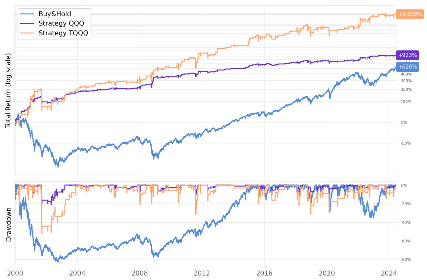
Next, quantitativo switched to the Nasdaq 100 Index ETF (QQQ) and the three-leveraged Nasdaq 100 ETF (TQQQ). The results show that performance on TQQQ was good (see previous figure):

Sharpe ratios reached 2.3 (QQQ) and 1.92 (TQQQ), which are quite good indicators for index targets (especially compared to China A-shares).

Improved Strategy: Adding Factors

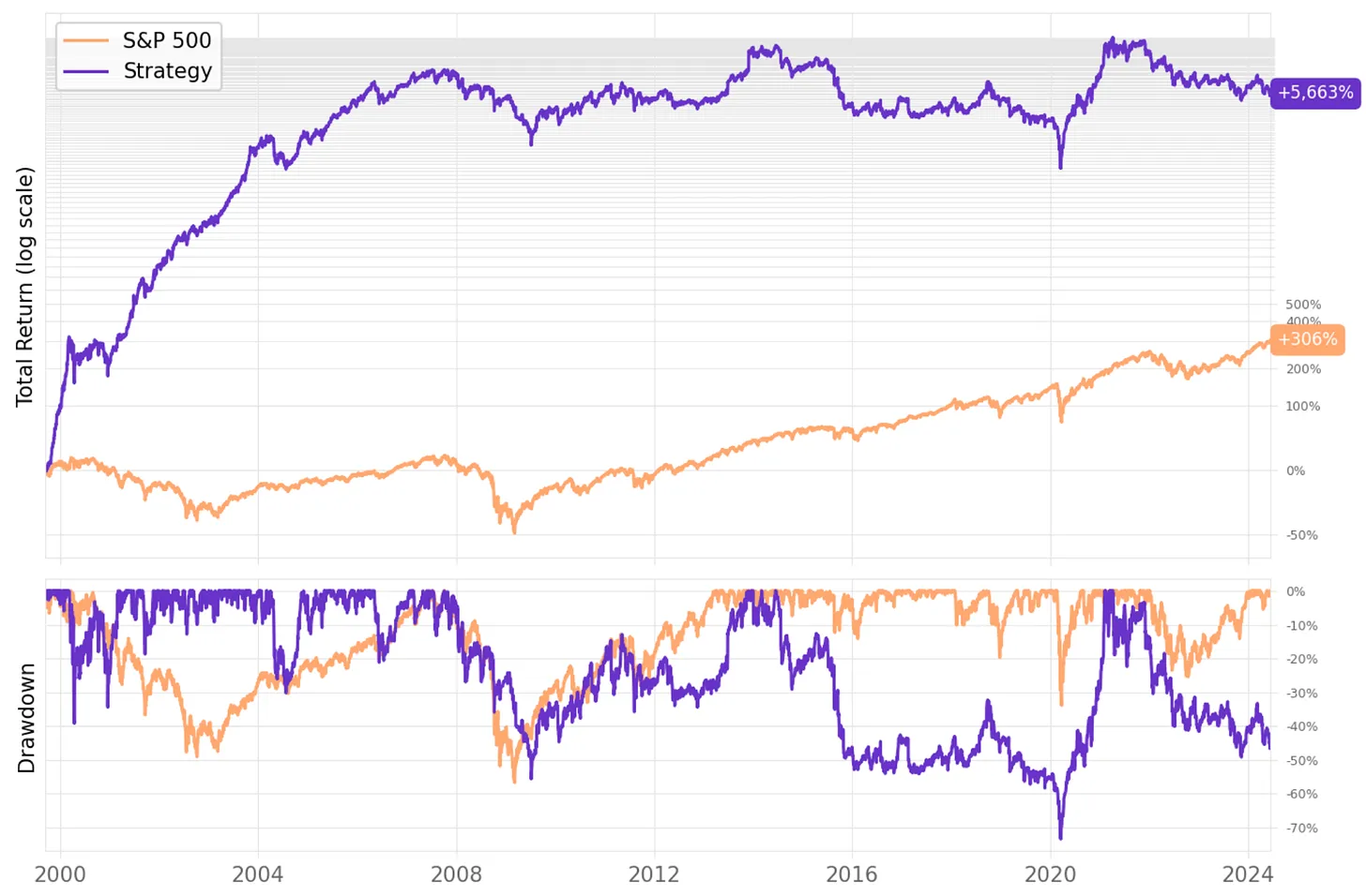
Based on the previous experiment, quantitativo added an asset portfolio.

They divided funds into ten parts (10 slots) to buy targets where the previous day's RSI closed below 5; if there are more than 10 targets in the universe triggering entry signals, they are ranked by market cap, prioritizing smaller-cap stocks. The exit condition is changed to the closing price falling below the target's 200-day moving average.

Additionally, they restrict trading only to targets with good liquidity:

1. Only trade targets that have not been suspended at all in the past 3 months
2. Do not include targets with a median daily trading volume in the past 3 months less than 20 times the fund share

---

The results this time are quite good, with an overall annual return rate of 17.8%, three times that of the benchmark. However, there is a problem: all of this was achieved in the first 8-9 years. The strategy stopped executing after 2008 and has since lost to the benchmark.

Why? By analyzing the 11,380 trades conducted during the 25-year backtest, quantitativo found many delistings. The problem with this naive approach is that the strategy prioritizes small-cap stocks (after passing the liquidity filter), which have a delisting probability of +70%.

Second Improvement: Reducing Delisting Risk

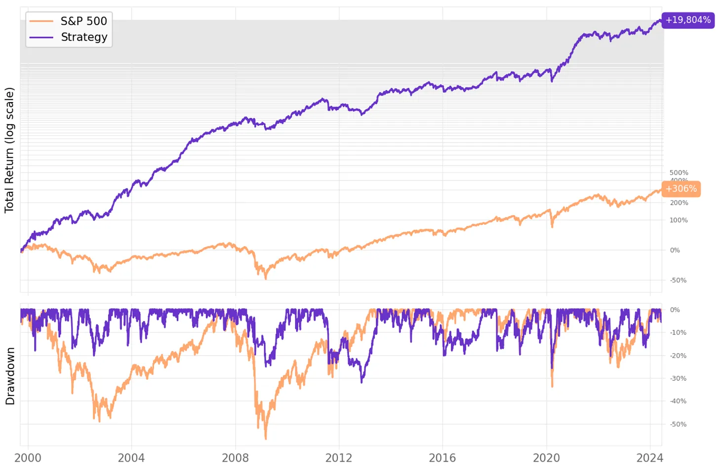
quantitativo improved the strategy again, this time by limiting the universe to trade only large and mega-cap stocks, which have lower delisting probabilities (35% and 9% respectively).

---

This time, the effect is obvious. The strategy's annualized return reached 23.9%, four times that of the benchmark during the same period, with a Sharpe ratio of 1.23% and a max drawdown of 32%, almost half that of the S&P 500. However, a pre-existing problem remains: the number of trades is too frequent. It still trades 461 times a year.

Third Improvement: Reducing Slots

The previous experiments used 10 slots, which was likely the main cause of the excessive number of trades. Thus, quantitativo reduced the number of simultaneously held targets to 2.

Now, the number of trades has decreased from 461 times/year to 90 times/year. And it achieves an annual return rate of 30.3%, five times that of the benchmark.

Conclusion

This article introduces a mean reversion strategy based on short-term RSI and, finally, provides an implementation with an annualized return of 30.3% (excluding slippage and trading fees).

The core of this strategy is short-term RSI. Although this indicator has been invented for over 45 years, the backtest results show that if you study something deeply enough, you are likely to succeed.

This solution is worth your reading time, but more importantly, we discussed the general process of strategy discovery and optimization angles.

---

Let's recap one more time as the closing remarks for this article:

1. RSI represents tides and regression, rooted in human nature, so it will never go out of style.
2. Multi-factor strategies can also be centered around a single factor, introducing other factors as restrictive conditions during trading.
3. The article provides a method to judge target liquidity strength, which you can also use as a factor.
4. The steps for developing strategies often start with single-factor testing, then writing simple backtests, and optimizing step-by-step based on backtest results.
5. In the optimization process, quantitativo first used ETFs, then switched to 10 slots, and finally returned to a 2-slot scheme.

---

Visible But Unattainable! 7 Years, 2500x Growth

This week, we continue to explore the use of the Alphalens factor analysis framework. The relationship between factors and returns is rarely linear, but Alphalens itself is a linear analysis framework, excelling at revealing linear relationships between factors and returns. The three analysis methods it supports are:

• Regression
• IC/Rank-IC (Correlation Coefficient, Rank Correlation)
• Tiered Regression (Layered Backtest)

All are based on linear regression or quasi-linear (compared to SVM, NN, etc.). Therefore, how to make Alphalens truly reveal the relationship between factors and returns in factor testing is a somewhat technical skill.

In our video account post on July 26, we explored how to use plot_quantile_statistics_table and the mean period wise return by Factor quantile chart to peel back the layers and reconstruct factors, ultimately perfectly revealing the linear relationship between factors and returns.

Here, we also provide a summary of the video content.

In the experiment, we first used 400 tickers and 1,000 days of data. After determining the experimental direction, we expanded to 2,000 tickers and 2,000 days of data to exclude chance.

---

The factor we are exploring is the 6-period RSI. As a factor, it is generally required that the larger the factor value, the higher the return; but RSI is exactly the opposite. It is generally believed that the larger the RSI, the more one needs to reduce positions. Therefore, the factor we actually construct is:

$$

factor = 100 - RSI

$$

First Experiment

Running Alphalens with default values simply yields the following results:

Long-short portfolio returns

Factor layering under default parameters

---

mpwr chart by quantiles

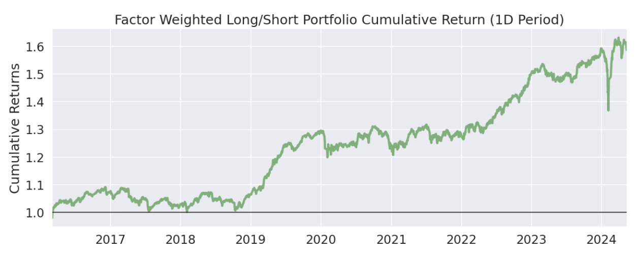
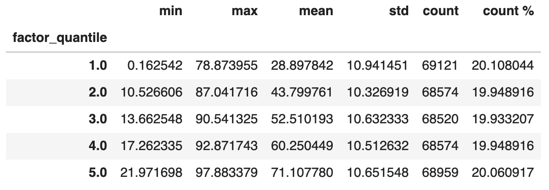
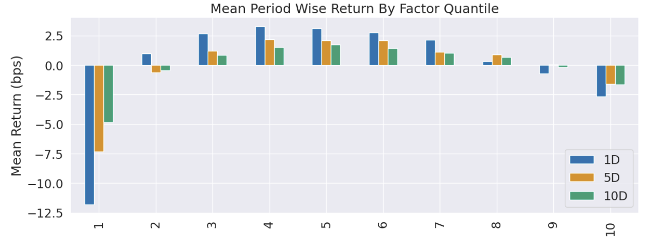
Looking at returns, there seems to be no problem. If you are doing pure data mining, you might think there's nothing wrong with it, since this factor is profitable, right?

But if we look closely at the layering chart, we will find that this experiment is meaningless. Because the factor value in the first layer spans from 0 to 78.9, and in the last layer, from 22 to 97.

Looking at the mean layering return chart, we will find no linear relationship between factors and returns. Since Alphalens can only do linear analysis, how can it reveal the causal relationship between factors and returns in this case?

Second Experiment

Alphalens's default layering method is by quantiles. We can use this method to layer only if the factor itself is uniformly distributed. RSI is not.

Besides RSI, there are many other examples unsuitable for by quantiles layering. For example, if the factor is corpus sentiment-based, the factor values might be labels like 0~5. In this case, layering by quantiles is also not suitable.

---

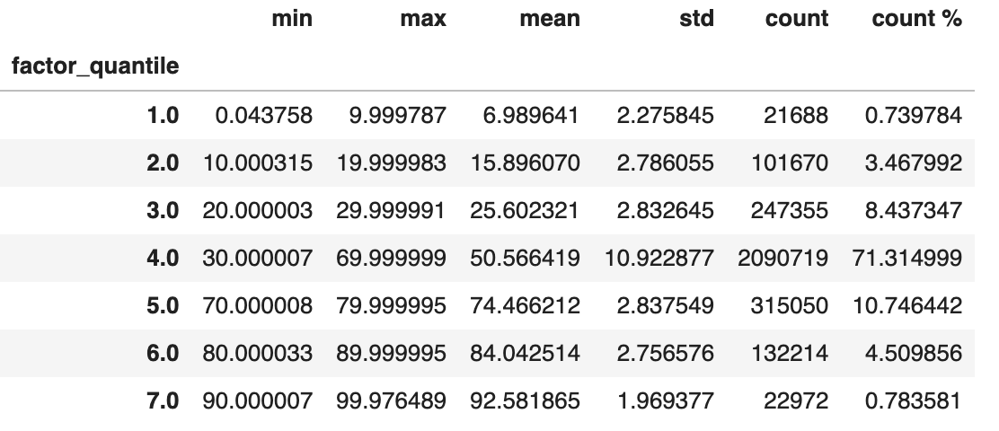
Alphalens provides another layering method, i.e., by bins. We provide bins as [0,10,20,30,70,80,90,100]. Here, we have an assumption that we are not interested in the middle RSI values, believing they will not provide trading signals.

Now the layering results are very reasonable:

Layering by bins

But if we look at the mean period wise return by Factor quantile chart, we will find a mirror-image linear relationship between factors and returns:

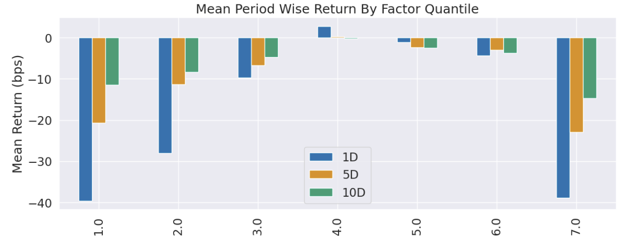
If Alphalens could go long on Group 4 and short on Group 1, the strategy results should be good. But Alphalens cannot do this. We need to modify the factor.

---

Our method is to discard the part of the factor values greater than 50, and then let Alphalens analyze whether there is a relationship between factors and returns.

Third Experiment

This time, we obtained a very perfect linear relationship:

Filtering out part of the factors

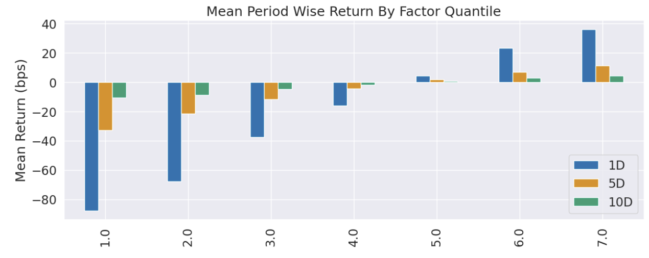
In this case, we can consider Alphalens's analysis results to be valid.

Of course, the returns are also very good.

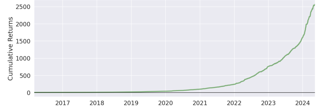
Too good to be true. Only the limit-up factor can surpass this strategy.

---

Discussion on Returns

Generally, when we see such good returns, we should consider that there might be an implementation issue. Is there an implementation issue in our experiment? Factor analysis is complex, which is why we try to use frameworks as much as possible. If you use the right framework, you must accept even the most bizarre conclusions.

So, can we cash in on these returns? Only a very few people can. Because most of its returns are achieved by shorting Group 1. In our algorithm, Group 1 is actually the group where RSI is greater than 90.

The stocks in this group are often limit-up stocks. Shorting is difficult under normal circumstances, and even more difficult now. However, from some违规 cases disclosed this year, some institutions first pull up limit-ups and then short via securities lending, fully utilizing the results of our factor analysis here: i.e., when RSI > 90, shorting has a high win rate.

Therefore, only a very few people can cash in on such high returns.

As various trading rules improve, the profits previously cut by these people will now return to the market.

Conclusion

Alphalens cannot reveal complex nonlinear relationships due to its factor testing methodology. Therefore, for factors where the relationship with returns is not simply linear, we must apply appropriate transformations to fit the analytical framework.

Otherwise, regardless of whether your factor is good or bad, you will not obtain correct results.

---

Top Quantitative Investing Journals (Part 1)

1. Journal of Finance was founded in 1946 and is a premier academic journal published by the American Finance Association. It attracts submissions from top scholars worldwide and serves as a key metric for academic achievement and career development. Many early works by Nobel laureates in Economics were published here, including Modern Portfolio Theory (Markowitz), the Capital Asset Pricing Model (William Sharpe), the MM Theorem (Merton H. Miller), and the Efficient Market Hypothesis (Eugene Fama).
2. Journal of Financial Economics. Rolf Banz published The relationship between return and market value of common stocks (the small-cap factor) in 1981 in this journal. In 2015, Fama’s five-factor model was also published here.
3. Review of Financial Studies, published by Oxford, is a peer-reviewed academic journal. Its impact factor was 5.814 in 2020, ranking 5th out of 110 in business and finance. The paper Market Liquidity and Funding Liquidity was first published here. On Google Scholar, it has over 6,500 citations.
4. Journal of Portfolio Management, focusing on the practice and theory of portfolio management, including quantitative strategies and risk management.
5. Journal of Financial and Quantitative Analysis (JFQA), publishing theoretical and empirical research in finance and economics.
6. Journal of Empirical Finance, emphasizing empirical research, including empirical analyses of market efficiency, asset pricing, and investment strategies.
7. The Journal of Trading, a journal focusing on trading strategies, market dynamics, and trading techniques, though it has ceased publication. Similar magazines include The Traders' Magazine.