
Second-Derivative Momentum Factor: 61.5% Alpha in China A-Shares
The previous Important Calendar warned that this week is "Super Central Bank Week," compounded by US tech earnings reports, creating significant volatility. Indeed, global equities suffered severe shocks this week. Intel plummeted over 26% in a single day.
This Week's Highlights
- US July non-farm payrolls missed expectations, triggering the Sam Rule; the Fed held off on rate cut decisions.
- The Bank of Japan raised interest rates, triggering a global stock market sell-off. Oil and the US dollar dropped sharply, while the RMB surged by nearly 1,000 points.
- Financial sector crackdown: Dong Guoqun, Chen Xiaopeng, and others are under investigation.
- NVIDIA's Blackwell chip defects delay mass production.
Next Week's Watchlist
- Monday: Caixin releases PMI data; Friday: National Bureau of Statistics releases CPI/PPI.
- Weight-loss giants Novo Nordisk and Eli Lilly will both report quarterly earnings next week.
- Construction machinery giant Caterpillar and entertainment giant Disney will report earnings next Tuesday and Wednesday, respectively.
This Week's Selection
- Second-Derivative Factor Generates Alpha 61.5%! (Paid article on WeChat Official Account)
- TradeGPT! Generate Trading Strategies with ChatGPT!
- Awesome! New Tool for Asset News Sentiment Analysis
- Where Do You Download Papers? Two Websites Recommended, Fast!
News Review
- US July Non-Farm Payrolls Miss Expectations, Sam Rule Triggered, Fed Holds Off on Rate Cuts
US Department of Labor data shows US non-farm payrolls added 114,000 in July, with wage growth slowing to 3.6%, a three-year low. Meanwhile, the unemployment rate rose from 4.1% to 4.3%, triggering the Sam Rule, which predicts recessions.
At last week's Federal Reserve meeting, the Fed decided to keep the benchmark interest rate in the 5.25%~5.50% range. Since there are no regular Fed meetings in August and October, the September meeting will be crucial.
Powell stated that if the US economy develops as expected, the Fed might cut rates as early as September. Regarding the Sam Rule, Powell acknowledged it, calling it a statistical pattern. However, some analysts believe the July non-farm data was affected by seasonal hurricanes. - BOJ Rate Hike, US Tech Earnings, and Weak Non-Farm Data Trigger Global Stock Sell-Off. The Nikkei fell 5.81% on Friday, and the Nasdaq dropped 2.43%. Intel plummeted over 26%, and it predicted Q3 revenue below expectations, announcing layoffs of 15,000 workers. Other tech stocks that dropped significantly include Amazon (-8.78%) and ASML (-8.41%). Oil fell 3.41% on Friday, the US Dollar Index against six major currencies dropped 1.15%, and the RMB rose by 873 points.
- Financial Sector Crackdown: Former SSE Vice President Dong Guoqun and Chen Xiaopeng, former Party Secretary and Director of the CSRC Shenzhen Regulatory Bureau, are under investigation. Haitong Securities announced that Vice President Jiang Chengjun has resigned.
- NVIDIA's Blackwell Chip Defects Delay Mass Production, involving billions of dollars in chip orders. Meanwhile, NVIDIA faces an antitrust investigation from the US Department of Justice.
- Vitamin Prices Soar After BASF Explosion: Due to a sudden explosion at BASF's plant in Germany, Vitamin A prices surged 53% in two days, and Vitamin E prices rose 20%. On August 1, BASF (China) told Securities Times reporters that it is currently impossible to assess when production will resume.
Second-Derivative Factor Generates ALPHA 61.5%!
In this issue, we introduce a second-derivative factor. We will demonstrate the exploration and optimization process of the second-derivative factor, further explaining the principles of factor analysis, including:
- How to use custom layered backtest (quantiles/bins) in Alphalens.
- The mathematical principles of the second-derivative momentum factor.
- What "layering" actually means: By quantiles or By bins.
Finally, in a 40% sample of China A-shares, we found that the optimal parameter for the second-derivative factor over the last six months is 5 days. Under this parameter, the annualized Alpha is 38.4% (long-short) and 61.5% (long-only), with a beta of -0.12, indicating returns are independent of the market.
In the previous issue, we examined the slope factor. Essentially, the slope factor is a first-derivative momentum factor. For example, for an array generated as follows, its slope and first derivative are equal:
from scipy.stats import linregress
slope = 0.2
x = np.arange(10)
y = slope * x + 1
d1 = np.diff(y).mean()
# If we calculate the slope via linear regression
alpha, beta, *_ = linregress(x, y)
print(f"slope is {slope:.1f}")
print(f"first derivative is {d1:.1f}")
print(f"slope by linear regression is {alpha:.1f}")All three outputs are 0.2. If we calculate the second derivative of the price series as a factor, does it predict future trends? Let's look at the results first, then discuss the underlying principles.
Second-Derivative Momentum Factor Testing
The following code generates a second-derivative momentum factor.
def d2_factor(close: NDArray, win: int = 10) -> NDArray:
n = len(close)
d1 = close[1:]/close[:-1] - 1
d2 = d1[1:] - d1[:-1]
factor = move_mean(d2, win)
# Left-pad to match input length
factor = np.pad(factor, (n-len(factor), 0), ...)
return factorNote that we use close[1:]/close[:-1]-1 instead of the standard first derivative to achieve a form of standardization. If we didn't do this, the factor for high-priced stocks would always be larger than that for low-priced stocks, leading to permanent higher factor exposure.
The factor's parameter is win, representing the time window over which the second derivative is calculated.
We then use Alphalens for factor testing. For the first call to Alphalens, we use quantiles for layering, with 10 layers.
From the layering chart, it is meaningless to proceed with return analysis; we must optimize first.
First Optimization
Considering that long returns peak at the 8th layer, we consider dropping the 9th and 10th layers to analyze the results.
Generally, Alphalens analysis involves three steps:
- Construct the factor.
- Data preprocessing, usually via
get_clean_factor_and_forward_returns. - Call
create_full_tearsheetto execute factor testing and output reports. Its input is the output from step 2.
Alphalens performs layering in step 2. It then uses the output from step 2 as the input for step 3.
Therefore, after obtaining the output from step 2, we can drop the 9th and 10th layers and call create_full_tearsheet for return analysis. This way, in Alphalens' view, the top layer is now the 8th layer, and all analysis is based on this.
This is allowed according to Alphalens' official documentation.
The output of step 2 is a DataFrame with the following format:
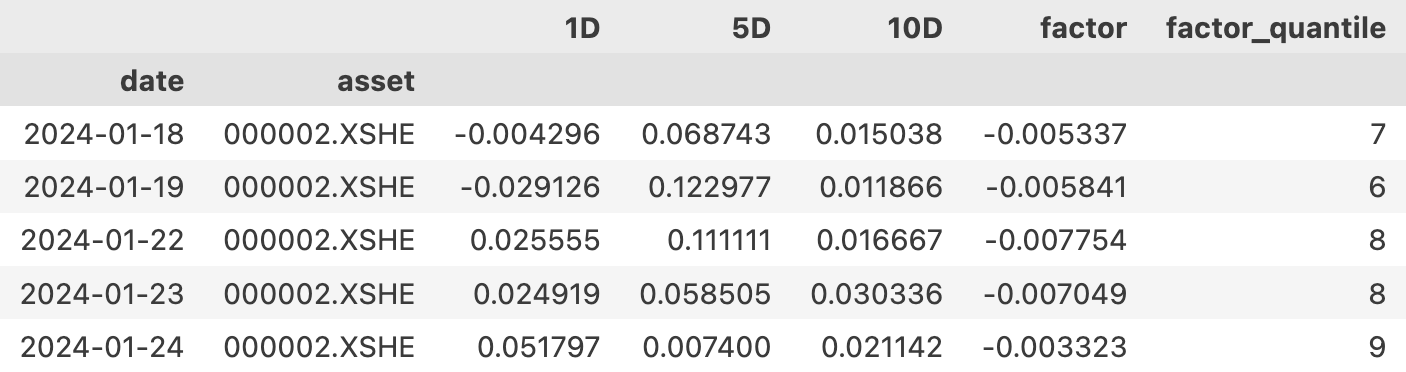
Thus, to drop the 9th and 10th layers, we can do:
factor_data = factor_data[factor_data.factor_quantile <= 8]tip
This is the first technique introduced in this article. In previous courses, to make Alphalens perform return analysis according to our specified layering, we used methods to modify the factor itself, which is earlier in the stage. Both methods are usable, but this one is simpler.This time, we obtained a satisfactory layering return mean chart: monotonic and increasing, fully suitable for further factor analysis.
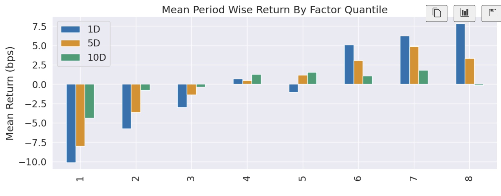
This chart essentially reproduces the previous one, just missing the 9th and 10th layers. However, now the 8th layer becomes the top layer, which is the layer Alphalens will long when calculating long-short returns.
tip
Since we can also drop the 9th and 10th layers in **live trading**, this operation is reasonable. Similar techniques can be seen in Alpha101.Pure Long Scenario
In previous issues, we discussed that due to institutional factors, not everyone can short-sell. So, let's see how the factor performs in a pure long scenario.
This time, annualized Alpha is only 17.6%, with a beta of -0.6. However, cumulative returns over 7 months are around 15%, slightly higher.
| Condition | Alpha | Beta | Cumulative Return |
|---|---|---|---|
| Long-Short, 10 | 23.2% | -0.07 | 11% |
| Long-Only, 10 | 17.6% | -0.60 | 15% |
Comparing the cumulative return charts of the two scenarios, we can see that the long-short portfolio has lower absolute returns but stronger risk-mitigating capabilities:
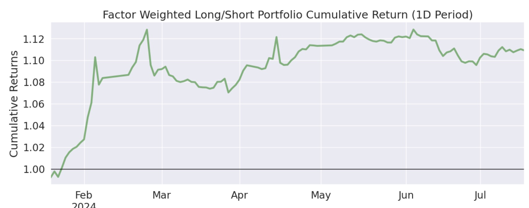
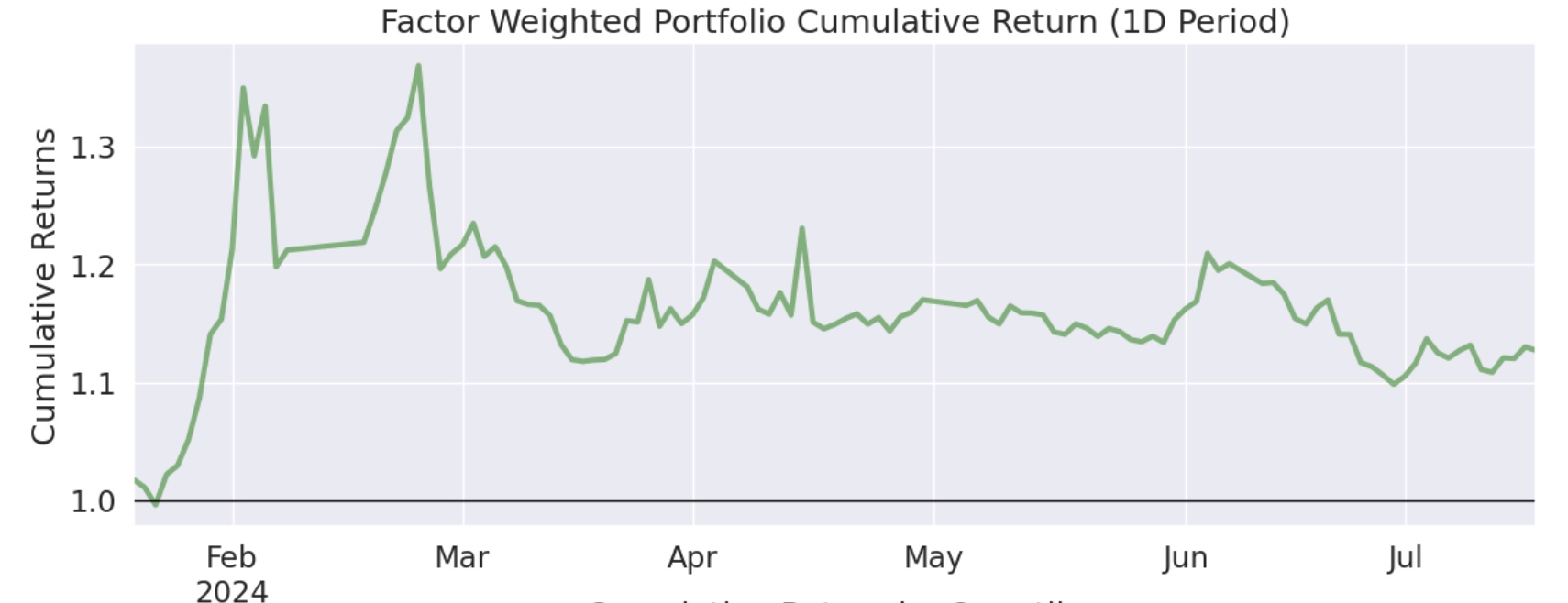
Why is the Alpha of the long-short portfolio greater than pure long, yet its cumulative return is lower than long-only? This may be due to some negative effects during the short-selling of the second-derivative factor. Some strong stocks, after a sharp drop (negative second derivative), often have a small rebound. If we short-sell just before this small rebound, it results in losses.
Finding the Most Effective Window
So far, we have used a 10-day window to calculate the second derivative. What if we use other windows? We tested data for 2, 4, 6, and 8 days. Now, let's summarize all the data:
| Condition | Alpha | Beta | Cumulative Return |
|---|---|---|---|
| Long-Short, 2 | 30.6% | -0.06 | 15% |
| Long-Short, 4 | 35.3% | -0.1 | 17% |
| Long-Short, 5 | 38.4% | -0.12 | 19% |
| Long-Short, 6 | 37.3% | -0.12 | 18% |
| Long-Short, 8 | 32.4% | -0.06 | 14.8% |
| Long-Short, 10 | 23.2% | -0.07 | 11% |
| Long-Only, 10 | 17.6% | -0.60 | 15% |
| Long-Only, 5 | 61.5% | -0.58 | 37% |
It appears that on the China A-shares market, the second-derivative momentum factor performs best with a period of 5. At this point, if we can construct a long-short portfolio, the annualized Alpha is 38.4%, and year-to-date cumulative returns are 19%; if we can only construct a long-only portfolio, the annualized Alpha is 61.5%, and year-to-date cumulative returns are 37%.
A Review of High School Math
The slope factor (i.e., first-derivative factor) discussed in the previous issue reflects the speed of price increase.
So, what does the second-derivative factor represent?
The second-derivative factor reflects the acceleration of price changes.
When the first derivative is positive and the second derivative is negative, prices will still rise, but the trend slows down, and a trend reversal may occur. The converse is also true. The following formula shows a function with a second derivative:
$$ y = a x^2 + b x + c $$
When $a$ and $b$ take values between [-1, 0, 0, 1] and [10, 10, -10, -10] respectively, we get the following graph:
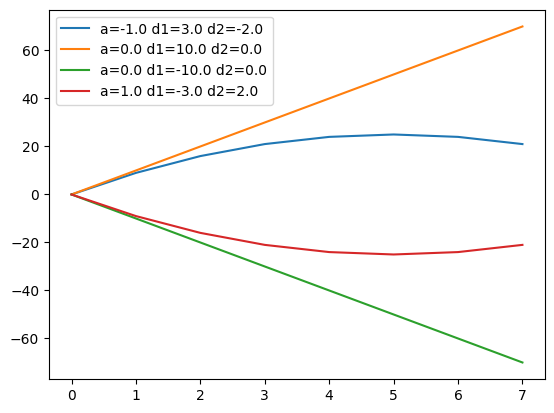
This graph illustrates that the second derivative has a corrective effect on the trend of security prices. A stock in an uptrend, if the second derivative remains negative, will eventually reach a peak and then turn downward; conversely, a stock in a downtrend, if the second derivative remains positive, will eventually hit a bottom and then turn upward.
Because of this, unlike the first derivative, the second derivative has the ability to predict changes in price trends in advance. It is a form of mean reversion momentum.
In the tests, the best-performing parameter was 5 days. Considering that the second derivative requires two additional windows to calculate, we actually generate trading signals based on the past 7 days of data.
7 days, this is the golden number.
Seeing Is Believing
Seeing an Alpha of 38%, I must admit, was surprising.
Is this real? Or has some Pseudo-Logoi (the god of lies) sneaked in somewhere?
Although we can trust Alphalens as a quality guarantee, you might prefer to believe your own "Cazilan big eyes" (a Chinese internet slang for clear vision) over a pile of statistical numbers.
Therefore, I decided to plot the price trends of individual stocks in the 8th layer. The plotting method is to first take all targets on a certain day (denoted as T0) with quantile = 8, and then take the closing prices for the most recent 8 days (up to T0). Before plotting, we normalize the starting point of the closing prices to 1.
In the plot, we used 199 samples, which is sufficient for representativeness and robustness.
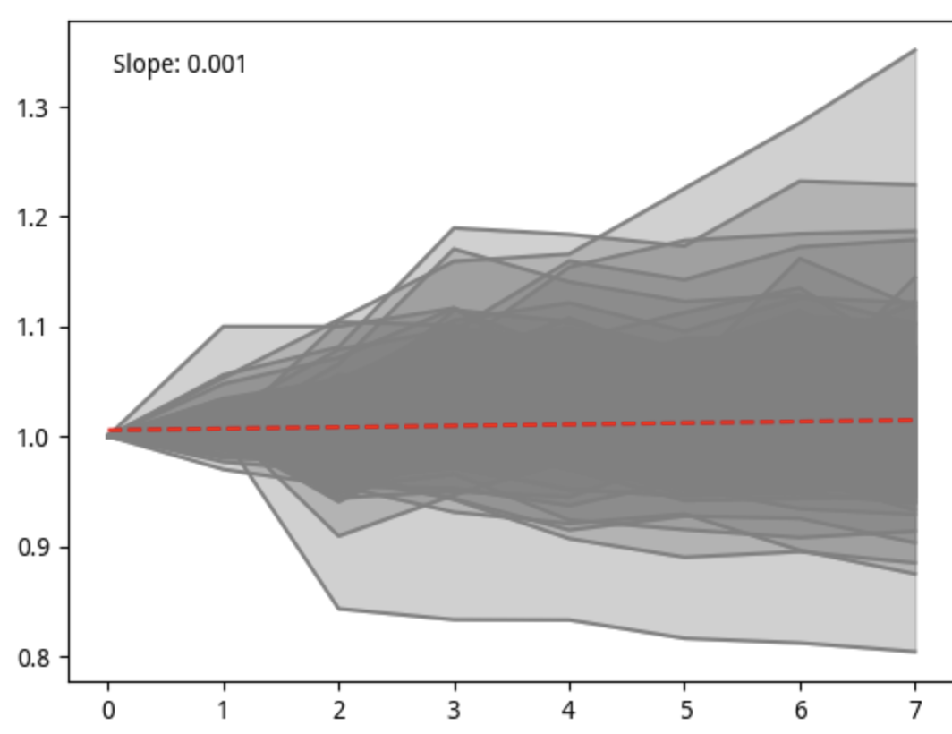
The red line in the chart is the trend line, with a slope of 0.001, indicating an overall upward trend; the depth of color represents the distribution density of the samples, showing that more samples are distributed above the zero line.
I like to draw inspiration from some stock market proverbs. Due to differences in company fundamentals, market mechanisms, and trading systems, copying overseas stock market practices is not feasible. The underlying game theory here is heavier.
Logically, the stock market proverbs related to the second-derivative momentum factor are golden pits and圆弧 tops (arc tops), or V-reversals. So, can we intuitively plot how many beautiful "golden pits" exist in these targets?
It is difficult to plot with a single chart and the same parameter: the period, depth, and construction stage of each golden pit are different. Like the beauty of Huan Fei and Yan Shou, it is hard to capture all the charm in one stroke.
By bins, or By quantiles?
In this test, we have always used by quantiles for layering, without exploring by bins layering.
By quantiles is a ranking-based layering. This is determined by the definition of quantiles. Using the by bins method, we focus more on the financial meaning of the factor value itself.
For example, for RSI, its value ranges from 0 to 100. Values above 80 are considered "overbought," and values below