This Week’s Highlights

• Fed Chair Powell states the time for a rate cut has arrived.
• JPMorgan significantly reallocates its Hong Kong stock positions, involving a market cap exceeding HK$1.1 trillion.

Next Week’s Watchlist

• The first "three-year holding period" fund managed by Guangfa’s star fund manager, Liu Geshan, is nearing maturity, with losses exceeding 58%.
• Thursday is the A50 index delivery date; Friday marks the month-end close.
• Saturday: Release of the official manufacturing PMI for August.

This Week’s Selection

• How to Implement Alpha 101?
• Efficient Quant Coding: Mask Arrays and Finding Runs
• Beyond In-Sample Testing: What Other Overfitting Detection Methods Are Available?

News Details

• Fed Chair Powell stated that the inflation rate is only half a percentage point above the Fed’s 2% target, and the unemployment rate is rising, indicating that "the time for policy adjustment has arrived." Cailian Press
• JPMorgan recently significantly reallocated its Hong Kong stock positions, involving a market cap exceeding HK$1.1 trillion. After the reallocation, the firm’s stockholding market cap ranking dropped from 4th to 14th, with holdings under HK$20 billion. One month prior, JPMorgan had also reallocated over HK$600 billion. Financial World
• The first "three-year holding period" fund managed by Guangfa Fund’s star fund manager, Liu Geshan, is nearing maturity. It raised an initial HK$14.87 billion. As of August 22 this year, the fund (A/C) has incurred losses exceeding 58% since inception. Recently, three-year holding period funds have been maturing in large numbers. Looking back, between 2021 and 2022, the public fund industry densely launched at least 73 three-year holding period active equity funds. After the lock-up period ends, will investors redeem in massive volumes? This is one of the most significant volatility factors next week. We believe relevant authorities are prepared.Sina Finance
• On August 25, Beijing Business Today marked the first anniversary of its commentary titled "Foreign Investors Ignore A-Shares Today, But Tomorrow They’ll Be Out of Their League." In that commentary from a year ago, Beijing Business Today pointed out that at a stage where stocks have extremely high investment value, some foreign capital flowing out of A-shares might represent typical technical traders who are anxious about index fluctuations. However, they will ultimately regret it; when they try to return, they will inevitably have to pay higher prices. As the saying goes, "Ignore A-shares today, but tomorrow they’ll be out of your league." The day after this commentary was published, the Shanghai Composite Index opened at 3,219 points. One year later, it closed at 2,854 points.

How to Implement Alpha 101?

In 2015, World Quant published the report 《101 Formulaic Alphas》, which contained 101 different stock selection factors. 80% of these factors were already being used in World Quant’s trading at the time. Following the report’s publication, it sparked significant discussion in the industry.

Currently, factor libraries generated based on Alpha 101 have become essential for almost all quantitative platforms, data providers, and quantitative institutions. Furthermore, inspired by this, some institutions have built even more factors on this basis, such as Guotai Junan’s Alpha 191. Both factor libraries have been implemented by institutions. For example, DolphinDB and JoinQuant both provide implementations for these two factor libraries.

This article introduces how to understand and implement 《101 Formulaic Alphas》. The content is excerpted from Lesson 8 of our course, "Factor Analysis and Machine Learning Strategies," and has been condensed due to space constraints.

Data and Operators in Alpha 101 Factors

Before implementing Alpha 101 factors, we must first understand the data and basic operators used in their formulas.

Alpha 101 factors are primarily constructed based on price and volume, with only a small minority using fundamental data, including market cap and industry classification data [^fundmental_data].

In price-volume data, Alpha 101 relies on the most primitive data: OHLC, volume (成交额), amount (成交量), and turnover (换手率). Based on this, it calculates returns (daily price changes) and vwap (volume-weighted average price).

The calculation methods for returns and vwap are as follows:

1234567# THE NUMPY WAY
vwap = bars["amount"] / bars["volume"] / 100
returns = bars["close"][1:]/bars["close"][:-1] - 1

# THE PANDAS WAY
vwap = df.amount / df.volume / 100
returns = df.close.pct_change()

In addition, understanding Alpha 101 requires understanding its common operators. There are approximately 30 operators in Alpha 101. Some, such as abs, log, sign, min, max, and mathematical operators (+, -, *, /), do not require explanation.

Below, we explain the operators that need clarification one by one.

Ternary Operator

The ternary operator exists in C programming but not in Python. This operator can be expressed as: "x ? y : z", which is equivalent to Python’s:

123456expr_result = None

if x:
    expr_result = y
else:
    expr_result = z

rank

In Alpha 101, there are two types of rank: one is cross-sectional, ranking all stocks in the universe at the same point in time; the other is time-series, ranking a single stock across its time series.

The cross-sectional rank directly calls DataFrame.rank. For example,

1234567891011import pandas as pd

data = {
    'asset': ["000001", "000002", "000004", "000005", "000006"],
    'factor': [85, 92, 78, 92, 88],
    'date': [0] * 5
}
df = pd.DataFrame(data).set_index('date').pivot(index=None, columns="asset", values="factor")

def rank(df):
    return df.rank(axis=1, pct=True, method='min')

In the code above, date is the index, column names are assets, and factor is their value. We can sort the factor values of each asset cross-sectionally using rank(axis=1). When using the axis=1 parameter, the index is not included in the sorting. pct=True indicates returning percentage ranks, while pct=False returns integer ranks.

Sometimes we also need to sort within a time series. In Alpha 101, this type of sorting is defined as ts_rank, distinguished from cross-sectional rank by the ts_ prefix. Henceforth, when we see the ts_ prefix, we should understand it in the same way.

1234from bottleneck import move_rank

def ts_rank(df, window=10, min_count=1):
    return move_rank(df, window, axis=0, min_count=min_count)

Here, we use move_rank from bottleneck, which is significantly faster than similar implementations in pandas and scipy. If implemented using pandas, the code would be:

12345def rolling_rank(na):
    return rankdata(na,method='min')[-1]

def ts_rank(df, window=10):
    return df.rolling(window).apply(rolling_rank)

Note that [-1] in line 3 is mandatory.

The usage of rank and ts_rank is most typical in the application of the alpha004 factor. This factor is:

123# ALPHA#4	 (-1 * TS_RANK(RANK(LOW), 9))
def alpha004(low):
    return -1 * ts_rank(rank(low), 9)

Here, the parameter low is a wide DataFrame with assets as columns and dates as the index, containing the daily lowest price. Let’s look at the results of calling rank and ts_rank sequentially on the parameter low. After examining a few examples, we can quickly understand the factor calculation process in Alpha 101.

1234567891011121314151617181920212223from bottleneck import move_rank
from IPython.core.interactiveshell import InteractiveShell
InteractiveShell.ast_node_interactivity = "all"

df = pd.DataFrame(
       [[6.18, 19.36, 33.13, 14.23,  6.8 ,  6.34],
       [6.55, 20.36, 32.69, 14.52,  6.4,  6.44 ],
       [7.  , 20.79, 32.51, 14.56,  6.0 ,  6.54],
       [7.06, 21.35, 33.13, 14.47,  6.5,  6.64],
       [7.03, 21.56, 33.6 , 14.6 ,  6.5,  6.44]], 
       columns=['000001', '000002', '000063', '000066', '000069', '000100'], 
       index=['2022-01-04', '2022-01-05', '2022-01-06', '2022-01-07', '2022-01-10'])

def rank(df):
    return df.rank(axis=1, pct=True, method='min')

def ts_rank(df, window=10, min_count=1):
    return move_rank(df, window, axis=0, min_count=min_count)

df
rank(df)

-1 * ts_rank(rank(df), 3)

Example outputs three DataFrames sequentially. We see that rank is executed row-wise, ranking stocks by their lowest price; ts_rank is executed column-wise, ranking the cross-sectional ranks of each stock, reflecting changes in the lowest position.

For instance, stock 000100 had a cross-sectional rank at the 33rd percentile on January 4, 2022. By January 10, its cross-sectional rank dropped to the 16.7th percentile.

After applying ts_rank, its final factor value on January 10 becomes 1, reflecting the fact that its cross-sectional rank decreased. Similarly, for stock 000001, its cross-sectional rank on January 4 was 16.7% (the lowest). On January 5, its rank increased to 50%, and its final factor value for that day was -1, reflecting the increase in its cross-sectional rank.

This group of operators includes, in addition to ts_rank introduced earlier, ts_max, ts_argmax, ts_argmin, and ts_min. These operators take two parameters: first, the time series (e.g., close or open), and second, the length of the sliding window.

Note that these operators must be performed on a sliding window to avoid introducing future data.

Other common statistical functions, such as min, max, sum, product, stddev, etc., although not prefixed with ts_, are also time-series operators, not cross-sectional ones. Since we have already detailed the usage of time-series operators through ts_rank, and their functions are well-known, we will omit them here.

delay

In Alpha 101, the delay operator is used to retrieve data from n days ago. For example,

12345678910def delay(df, n):
    return df.shift(n)

data = {
    'date': pd.date_range(start='2023-01-01', periods=10),
    'close': [100, 101, 102, 103, 104, 105, 106, 107, 108, 109]
}
df = pd.DataFrame(data)

delay(df, 5)

In this way, when calculating the factor on day 5, the close data used is from 5 days ago, i.e., the close at the original index 0.

correlation and covariance

correlation is the Pearson correlation coefficient between two time series over a sliding window. This operator can be implemented as:

12345def correlation(x, y, window=10):
    return x.rolling(window).corr(y).fillna(0).replace([np.inf, -np.inf], 0)

def covariance(x, y, window=10):
    return x.rolling(window).cov(y)

Note that here, although we only called rolling on x, when calculating the correlation coefficient, it has been verified that y is also slid over the same window.

scale

According to Alpha 101’s explanation, the purpose of this operator is to scale the elements of an array so that sum(abs(x)) = a, with the default a = 1. It can be implemented as:

12def scale(df, k=1):
    return df.mul(k).div(np.abs(df).sum())

decay_linear

The purpose of this operator is to linearly weight-decay elements in a time series of length d, so that their sum is 1, with later elements having higher weights.

1234def decay_linear(df, period=10):
    weights = np.array(range(1, period+1))
    sum_weights = np.sum(weights)
    return df.rolling(period).apply(lambda x: np.sum(weights*x) / sum_weights)

delta

Equivalent to dataframe.diff().

adv{d}

Simple moving average of volume over d days.

signedpower

signedpower(x, a) is equivalent to x^a.

Alpha 101 Factor Interpretation

This section is omitted.

Open-Source Alpha 101 Factor Analysis Library

The best way to fully explore the factors defined in Alpha 101 is to calculate all these factors based on historical data and backtest them using Alphalens or even backtrader. popbo implements such functionality.

Running this library requires installing alphalens, akshare, baostock, and jupyternotebook. Before conducting research, you need to download data and calculate factors according to its README file. Then, you can open research.ipynb to analyze the annual performance of each factor.

In our supplementary materials, we provide the complete source code for this project, which can be run in our course environment.

Efficient Quant Coding: Mask Arrays and Finding Runs

In many quantitative scenarios, we need to count how many times an event has occurred consecutively, such as consecutive price limits (up/down), N consecutive bullish days, or calculating streaks in Connor's RSI.

For example, to determine the maximum number of consecutive price-up limits in the following closing prices, or the longest N consecutive bullish days, how should we calculate it?

12a = [15.28, 16.81, 18.49, 20.34, 21.2, 20.5, 22.37, 24.61, 27.07, 29.78, 
     32.76, 36.04]

Assuming we set a 10% price increase limit, we can convert the above array to:

12pct = np.diff(a) / a[:-1]
pct > 0.1

We obtain the following array:

1flags = [True, False, True, False, False, False, True, False, True, True, True]

This still cannot calculate the maximum number of consecutive price-up limits, but it is a basic data structure for many such problems. After converting the original data into a similar array based on conditions, we can use the following tool:

12345678910111213from numpy.typing import ArrayLike
from typing import Tuple
import numpy as np

def find_runs(x: ArrayLike) -> Tuple[np.ndarray, np.ndarray, np.ndarray]:
    """Find runs of consecutive items in an array.
    """

    # ensure array
    x = np.asanyarray(x)
    if x.ndim != 1:
        raise ValueError("only 1D array supported")
    n = x.shape[0]

1234567891011121314151617181920212223    # handle empty array
    if n == 0:
        return np.array([]), np.array([]), np.array([])

    else:
        # find run starts
        loc_run_start = np.empty(n, dtype=bool)
        loc_run_start[0] = True
        np.not_equal(x[:-1], x[1:], out=loc_run_start[1:])
        run_starts = np.nonzero(loc_run_start)[0]

        # find run values
        run_values = x[loc_run_start]

        # find run lengths
        run_lengths = np.diff(np.append(run_starts, n))

        return run_values, run_starts, run_lengths


pct = np.diff(a) / a[:-1]
v,s,l = find_runs(pct > 0.099)
(v, s, l)

The output result is:

1(array([ True, False,  True]), array([0, 3, 6]), array([3, 3, 5]))

The output result is a tuple consisting of three arrays, representing:

value: unique values start: start indices length: length of runs

In the output above, v[0] is True, indicating the start of a series of price-up limits, s[0] is the corresponding starting position (index 0), and l[0] indicates that the consecutive number of price-up limits is 3. Similarly, we can see that the longest consecutive price-up limit (v[2]) in the original array is 5 (l[2]), starting from index 6 (s[2]).

Therefore, to find the maximum number of consecutive price-up limits in the original sequence, we only need to find the maximum value in l. However, solving this problem still requires a technique: using the mask array introduced in Chapter 4.

123v_ma = np.ma.array(v, mask = ~v)
pos = np.argmax(v_ma * l)
print(f"最大连续涨停次数{l[pos]}，从索引{s[pos]}:{a[s[pos]]}开始。")

Here, the role of the mask array is to prevent data where v == False from participating in the calculation (v_ma * l) while preserving the order (indices) of these elements, so that when we later call the argmax function, the found index corresponds to the positions in v, s, and l.

The v_ma we created is a mask array with the value:

123masked_array(data=[True, --, True],
            mask=[False,  True, False],
            fill_value=True)

When multiplied with another integer array, True converts to the number 1, so the multiplication result is still a mask array:

123masked_array(data=[3, --, 5],
             mask=[False,  True, False],
            fill_value=True)

When arg_max is applied to a mask array, it ignores elements where the mask is True but preserves their positions. Therefore, the final result for pos is 2, corresponding to the element values in v, s, and l as: True, 6, 5.

To count the longest N consecutive bullish days? This is an easier task than finding price-up limits. However, this time, we will not use a mask array to implement it:

1234v,s,l = find_runs(np.diff(a) > 0)

pos = np.argmax(v * l)
print(f"最长N连涨次数{l[pos]}，从索引{s[pos]}:{a[s[pos]]}开始。")

The output result is: the longest N consecutive bullish days is 6, starting from index 5:20.5.

The key here is that when Numpy performs multiplication, True is treated as the number 1, and False as 0. Thus, the multiplication result naturally eliminates parts without consecutive bullish days, not interfering with the argmax calculation.

Of course, using a mask array may be semantically clearer, although mask arrays are slightly slower. However, correctness and readability are often more important.

Calculating Streaks in Connor's RSI Connor's RSI (Connor's Relative Strength Index) is a technical analysis indicator developed by Nirvana Systems as an improved version of the Relative Strength Index (RSI).

The main difference between Connor's RSI and traditional RSI is that it considers the number of consecutive days of price increases or decreases, known as "winning streaks" and "losing streaks." This consideration allows Connor's RSI to better reflect the strength of market trends.

After introducing the find_runs function, calculating streaks becomes very simple.

12345678910111213def streaks(close):
    result = []
    conds = [close[1:]>close[:-1], close[1:]<close[:-1]]

    flags = np.select(conds, [1, -1], 0)
    v, _, l = find_runs(flags)
    for i in range(len(v)):
        if v[i] == 0:
            result.extend([0] * l[i])
        else:
            result.extend([v[i] * x for x in range(1, (l[i] + 1))])
            
    return np.insert(result, 0, 0)

This code first divides the stock price series into three sub-series: rising, falling, and flat. Then, it calculates the number of consecutive rising or falling days for each sub-series and merges the results into a new array.

In the streaks, consecutive rising days are represented by positive numbers, and consecutive falling days by negative numbers. Therefore, in line 5, np.select is used to convert the condition array into a sequence of [1, 0, -1], and subsequent multiplication yields the correct number of consecutive rising (falling) days.

Beyond In-Sample Testing: What Other Overfitting Detection Methods Are Available?

I saw a humorous post on Zhihu claiming that someone, to make backtest results look better for selling strategies, planted numerous if statements in the code to check if the current date is a specific date, and then refrains from trading. The trick lies entirely within these dates, as trading on these dates is always losing.

The authenticity of this content is questionable. However, it is a typical example of overfitting.

Overfitting and Detection Methods

Overfitting refers to a model fitting the data so well that it cannot generalize, thus failing to work on another dataset. From a trading perspective, overfitting "designs" a strategy that trades historical data well but will definitely fail on new data.

Overfitting is our number one enemy in backtesting. How do we detect overfitting?

An obvious detection method is out-of-sample testing. It involves dividing the entire dataset into non-overlapping training and testing sets, training the model on the training set, and validating it on the testing set. If the model performs well on the testing set, we consider that the model is not overfitted.

When the sample size itself is insufficient, out-of-sample testing becomes difficult. Thus, people have invented some extended versions.

One such extended version is k-fold cross-validation, a common concept in machine learning.

It randomly divides the dataset into K subsets of roughly equal size. For each round of validation, one subset is selected as the validation set, and the remaining K-1 subsets are used as the training set. The model is trained on the training set and evaluated on the validation set. This process is repeated K times, and the final evaluation metric is usually the average of the K validation results.

This process can be simply represented by the following diagram:

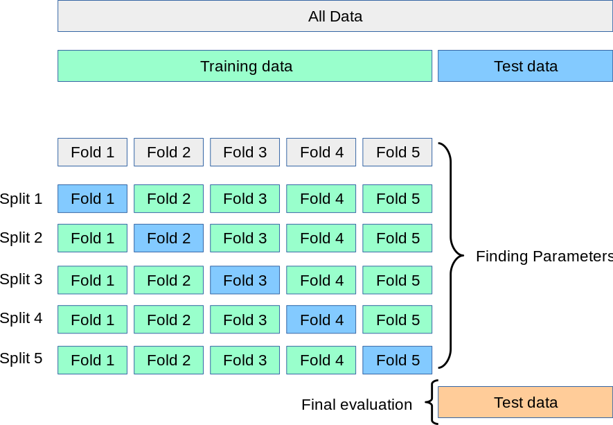
However, in time series analysis (typical in securities analysis), the k-fold method is not suitable because time series analysis has a strict sequential order. Therefore, a specialized version of k-fold cross-validation, called rolling forecasting, has been developed. You can view it as a sequential version of k-fold cross-validation.

It can be simply represented by the following diagram:

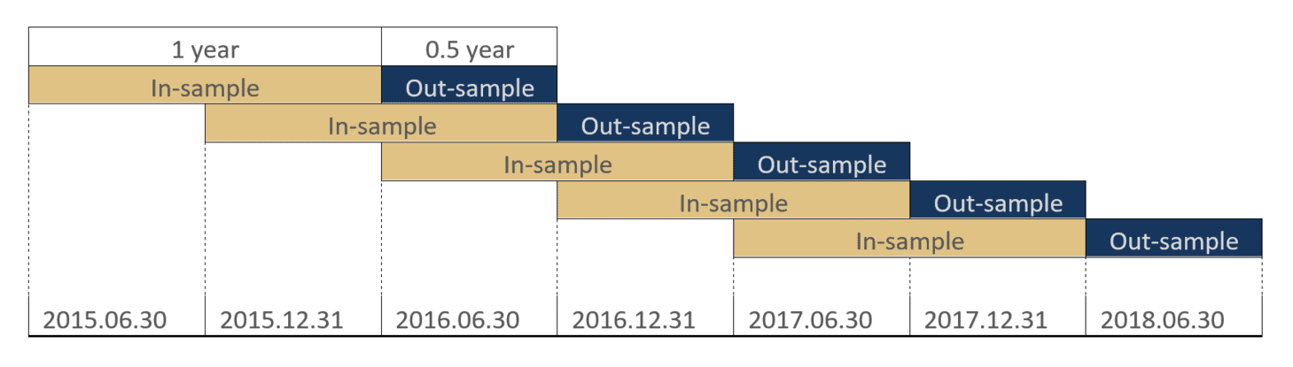
Comparing the two diagrams from k-fold cross-validation to rolling forecasting, the difference lies in that one is unordered, while the other emphasizes time order, with the training set and validation set needing to be continuous.

Sometimes, you may also see the term Walk-Forward Optimization. It is essentially the same as rolling forecasting.

However, I recently learned about a novel method from the buildalpha website: noise testing.

New Attempt: Noise Testing

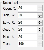
Buildalpha’s noise testing involves adding a certain ratio of random noise to backtest data, then performing backtesting, and comparing the backtest based on noise with the backtest based on real data.

Its principle is that during backtesting, historical data is only one possible path. If time were to repeat, history might not change its overall direction, but randomness would alter its pace. A good strategy should be able to withstand randomness and grasp the overall direction of history. Therefore, adding some clever noise to a time series might invalidate overfitted strategies, while truly effective strategies will still shine.

Buildalpha is a platform similar to TradingView. To perform noise testing, configuration can be done via a graphical interface.

Through this dialog box, buildalpha modified about 20% of the data, and the modification amplitude for OHLC was controlled within 20% of ATR. The "100" at the bottom indicates that we will randomly generate 100 sets of noisy data.

Let’s compare real data with data overlaid with noise.

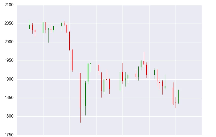
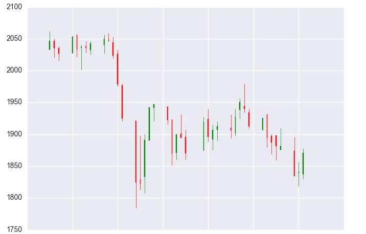
The left image shows real data, and the right image shows data with some noise overlaid. After adding noise, randomness is introduced in some details, but the stock price trend is not changed (the overlay is independent). If the stock price trend were changed, this method would be invalid or even harmful.

Finally, backtesting results for the same strategy are compared as follows:

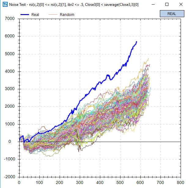
From the results, among the multiple possible paths in history, none of the backtest results are better than those based on real data.

In other words, the reason the real backtest results are so good is purely because the person formulating the strategy had a God’s-eye view, traveling back from the future.

Factor Robustness: Parameter Plains and Noise Testing

Factor robustness hinges on parameter stability. This article explores parameter plains and noise testing to identify overfitting and ensure strategy resilience.

Tags: Factor Testing, Overfitting, Backtest, Robustness

Parameter Plains and Noise Testing

Noise testing involves slightly perturbing historical data to assess robustness. In contrast, parameter plains offer a different approach to detecting overfitting: they examine whether minor adjustments to strategy parameters cause drastic changes in backtest performance. If performance remains stable under such perturbations, the strategy parameters are considered robust.

Build Alpha provides visual detection of parameter plains.

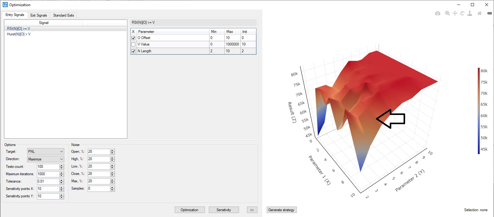
In this 3D plot, the selected parameters are X=9 and Y=4, indicated by the black dot. Clearly, this region is near a sensitive area where strategy performance degrades sharply. Following traditional recommendations, we should instead select parameters X=8 and Y=8, where the surface is flatter.

While parameter plains often provide valid insights—since our chosen parameters are essentially functions of price changes—they are not price changes themselves. The most direct method to verify robustness is to ensure that strategy performance remains on a flat surface even when prices undergo slight variations.

However, because such plots are difficult to construct, Build Alpha still generates 3D visualizations where parameters serve as coordinates in an n-dimensional space and strategy performance as the value. Yet, instead of relying on a single historical dataset, these plots are based on a set of historical data: both the actual historical data and noise-augmented data.