
FFT for Stock Prediction: Decoding Market Cycles
This Week's Highlights
- Market rumors suggest a reduction in existing mortgage rates; real estate ETFs surged, but multiple stocks hit price limits before closing.
- China’s official manufacturing PMI for August stood at 49.1%, a 0.3 percentage point decline from the previous month.
- The State Administration for Market Regulation announced that Alibaba has completed its three-year rectification process.
- Tongkun Group released its first semi-annual report of the year, showing a 911.35% year-on-year increase, the highest net profit growth among companies that have already published their reports.
Next Week's Focus
- Will the rumor about reducing existing mortgage rates materialize?
- Caixin Manufacturing PMI release on Monday.
- The 2024 Low-Altitude Economy Development Conference will be held in Wuhu from September 6 to 8.
This Week's Selection
- Is the Main Force Entering? Research on Fast Fourier Transform and Stock Price Prediction
- Serialized! Essential Numpy Programming for Quants (1)
This Week's Highlights
- Market rumors suggest that relevant authorities are considering further reducing existing mortgage rates, allowing up to 38 trillion RMB in existing mortgages to seek refinancing, thereby reducing residents' debt burden and boosting consumption.
As of Saturday, these rumors have not been officially confirmed. - In August, the PMI was 49.1%, a 0.3 percentage point decline from the previous month. By enterprise size, the PMI for large enterprises was 50.4%, still above the critical point; the PMIs for medium and small enterprises were 48.7% and 46.4%, declining by 0.7 and 0.3 percentage points, respectively.
The August PMI was influenced by high temperatures and did not significantly exceed expectations. - On the afternoon of August 30, the State Administration for Market Regulation announced that Alibaba had completed its three-year rectification process with good results. Alibaba’s stock price has fallen by 70% from its peak in 2020.
- On Friday, Eastern Time, the three major US stock indices rose collectively. The Dow Jones Industrial Average rose 0.55% to 41,563.08 points, setting a new record high. The S&P 500 rose 1.01%, and the Nasdaq rose 1.13%. The Federal Reserve’s preferred July PCE inflation data basically met expectations. The market’s bet on a significant Fed rate cut in September decreased, but the market still expects a significant rate cut in November or December.
- E Fund’s Nasdaq 100 ETF released its 2024 interim report. Changzhou Investment Group holds a 5.92% share, becoming the largest holder. Despite a net value increase of 49.21%, the ETF still rose 14.91% this year. The ETF was issued in 2017 and currently has a net value of 3.16.
- Tongkun Group released its first semi-annual report of the year, achieving a net profit of 1.065 billion RMB, a 911.35% year-on-year increase, the highest net profit growth among companies that have already published their reports. During the reporting period, downstream demand for polyester filament industry improved significantly compared to the same period last year, with increased product sales and price spreads. The industry is generally in a recovery state. Overall, the electronics industry was the big winner, with revenue growth leading all sectors. The total revenue for the first half of the year was 1.59 trillion RMB, a 17.3% year-on-year increase.
Next Week's Focus
- Market rumors on Friday suggested that reducing existing mortgage rates is under consideration. Real estate ETFs surged immediately, while bank stocks plummeted in response. However, prices fell back at the close, and many stocks hitting price limits failed to hold. Next week, will this rumor be confirmed or refuted? It could have a significant impact on the market.
- Caixin Manufacturing PMI release on Monday.
- The 2024 Low-Altitude Economy Development Conference will be held in Wuhu from September 6 to 8.
- US August unemployment rate and non-farm payrolls report released on Friday.
Is the Main Force Entering? Research on Fast Fourier Transform and Stock Price Prediction
An undeniable fact: economic activity is cyclical. However, this fact seems to have been long ignored by the quantitative community. Whether in asset pricing theory or trend trading theory, we can hardly find a place for cycle research -- in the latter context, people prefer to use terms like "swing" rather than openly saying "cycle."
In this article, we will explore cycles in the stock market. We will use the Fast Fourier Transform (FFT) to decompose time series signals into frequency domain signals, identify main force capital through signal energy, and make some predictions based on their operational cycles. Finally, we present three hypotheses, one of which has been proven.
FFT - Time-Frequency Conversion
(Data acquisition part omitted).
We have obtained the Shanghai Composite Index over the past year. Obviously, it is a time series signal. The Fourier Transform is precisely designed to convert time series signals into frequency domain signals. In other words, the Fourier Transform can decompose the Shanghai Composite Index into a combination of several sine waves.
# 应用傅里叶变换
fft_result = np.fft.fft(close)
freqs = np.fft.fftfreq(len(close))
# 逆傅里叶变换
filtered = fft_result.copy()
filtered[20:] = 0
inverse_fft = np.fft.ifft(filtered)# 绘制原始信号和分解后的信号
plt.figure(figsize=(14, 7))
plt.plot(close, label='Original Close')
plt.plot(np.real(inverse_fft), label='Reconstructed from Sine Waves')
plt.legend()We obtained the following output:
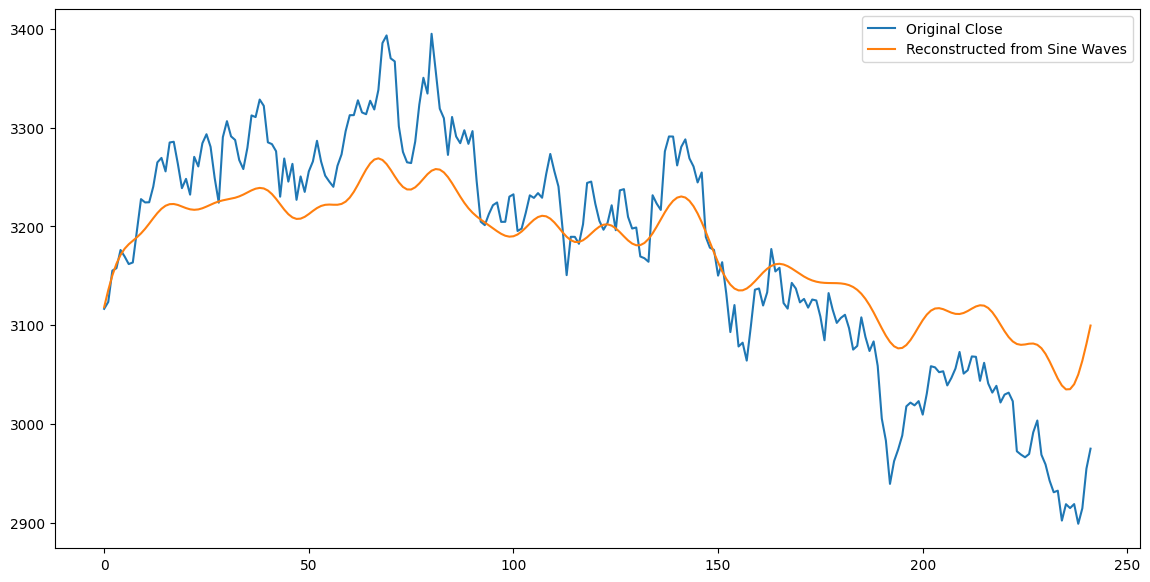
In the field of digital signal processing, time series are called time-domain signals, and after the Fourier Transform, we obtain frequency-domain signals. Time-domain signals and frequency-domain signals can be converted into each other. The fft library in Numpy provides fft and ifft functions to help us implement these two conversions.
np.fft.fft converts time-domain signals into frequency-domain signals. The result is a complex array representing the amplitude (i.e., energy) of each frequency component decomposed from the signal. Frequencies are arranged from low to high, with the 0th element having a frequency of 0, which is the DC component, a linear function of the signal's mean.
np.fft.ifft is the inverse transform of fft, converting frequency-domain signals back into time-domain signals.
Converting time-domain signals to the frequency domain reveals basic characteristics such as signal periodicity. We can also perform some operations on the frequency-domain signals obtained from the fft and then transform them back, which is digital signal processing.
High-Frequency Filtering and Compression
If we set the energy of high-frequency signals to zero and then inverse-transform the signal back, we will get a new sequence similar to the original sequence, but smoother -- this is what we often call low-pass filtering -- various moving averages you are familiar with are also low-pass filters.

In the above code, we only retained the energy of the first 20 low-frequency signals, resulting in a new sequence similar to the original sequence. If this method is applied in the image field, it achieves lossy compression -- the compression ratio is 250/20.
In the 1990s, the most advanced image compression algorithms were based on such principles -- retaining the mid-to-low-frequency parts of the image and treating high-frequency parts as noise to be removed, thereby preserving the main features of the image while significantly reducing the amount of data to be saved.
People working on such compression algorithms at that time all knew this beautiful young lady -- Lena. This photo is a standard test sample for image algorithms. Through long-term evolution, under the pressure of survival, humans have evolved super strong abilities to recognize others' expressions. Therefore, compared to other samples, once compression causes a decline in image quality, the human eye is more likely to detect changes in faces and expressions, making face images the best test samples.
 Lena
Lena
Lena is a model for Playboy magazine. This photo is a small part of her seductive photo taken for the November 1972 issue of Playboy -- in the original photo, Lena boldly displayed her seductive buttocks curve, but those unorthodox scientists only shared her smile with us -- from a scientific perspective, this is also the part with the highest information ratio.
Coincidentally, before Lena became the standard test sample for digital image processing, scientists were always using another young lady's photo, also from Playboy.
Okay, back to the topic. We just shared a method to remove high-frequency noise from signals, making the meaning of the signal itself more prominent. We also hope to use similar techniques in securities analysis to reveal signals hidden in K-lines.
But if we simply copy this method from other fields, it hardly counts as research, and it is difficult to achieve good results. In fact, in securities signals, we should pay more attention to signal energy compared to frequency, after all, we want to stand on the side of the most powerful people.
 May the Force be with you -- Star Wars
So, let's change our approach and keep the parts with the strongest energy in the decomposed frequency-domain signals to see what they look like.
Filtering Low-Energy Signals
# 保留能量最强的前 5 个信号
amp_threshold = np.sort(np.abs(fft_result))[-11]
# 绘制各个正弦波分量
plt.figure(figsize=(14, 7))
theforce = []
for freq in freqs:
if freq == 0: # 处理直流分量
continue
elif freq < 0:
continue
else:
amp = np.abs(fft_result[np.where(freqs == freq)])
if amp < amp_threshold:
continue
sine_wave = amp * np.sin(2 * np.pi * freq * np.arange(len(close)))
theforce.append(sine_wave)
plt.plot(dates, sine_wave, label=f'Frequency={freq:.2f}')
plt.legend()
plt.title('Individual Sine Wave Components')
ticks = np.arange(0, len(dates), 20)
labels_to_show = [dates[i] for i in ticks]
plt.xticks(ticks=ticks, labels=labels_to_show, rotation=45)
plt.show()The FFT gives frequencies in pairs of positive and negative. We can simply consider that negative frequencies are meaningless to us; they are a kind of dark energy we cannot see and need not care about. Therefore, in the code, we ignored this part.
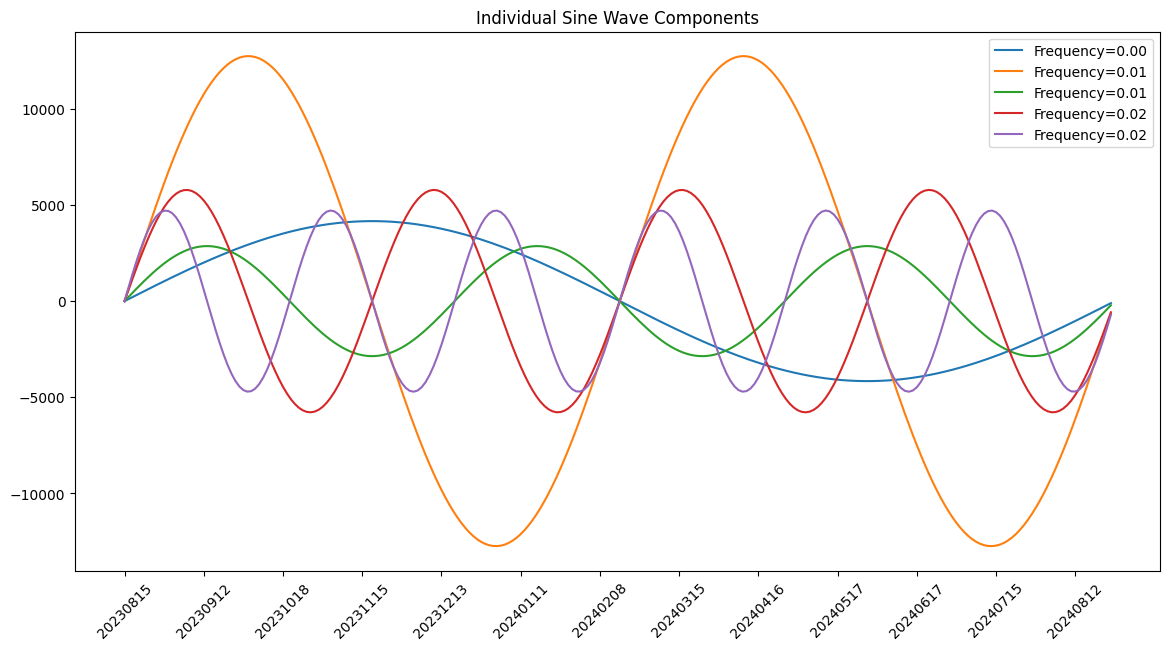
We see that the wave (orange) with the strongest impact on the Shanghai Composite Index trend has a cycle of about 7 months: it takes 3.5 months from peak to trough, and 3.5 months from trough to peak. Since its energy is almost double that of other waves, it dominates the trend of the entire superimposed wave: if other waves are in phase with it, the superimposed result will strengthen the trend; otherwise, it will offset the trend. The energies of other waves are similar, but their frequencies differ.
What exactly are these waves? They can be economic cycles, but ultimately, economic cycles are driven by people or reflect people's judgments. Therefore, we can view the cycle of fluctuations as the operational cycle of capital.
From this decomposition chart, we can hypothesize that there is long-term capital (corresponding to the blue wave) that rebalances once a year or so. There is medium-term capital (corresponding to the orange wave) that rebalances about every six months. Other capital is short-term, changing positions about every three months. There are countless high-frequency waves we filtered out, which operate frequently, possibly corresponding to retail investors, but their energy is small and can generally be ignored; only in extremely rare cases can they form superimposed effects in the same direction, thereby affecting the trend.
Now, let's synthesize the operations of these capital flows and compare them with the actual trend to see how it goes:
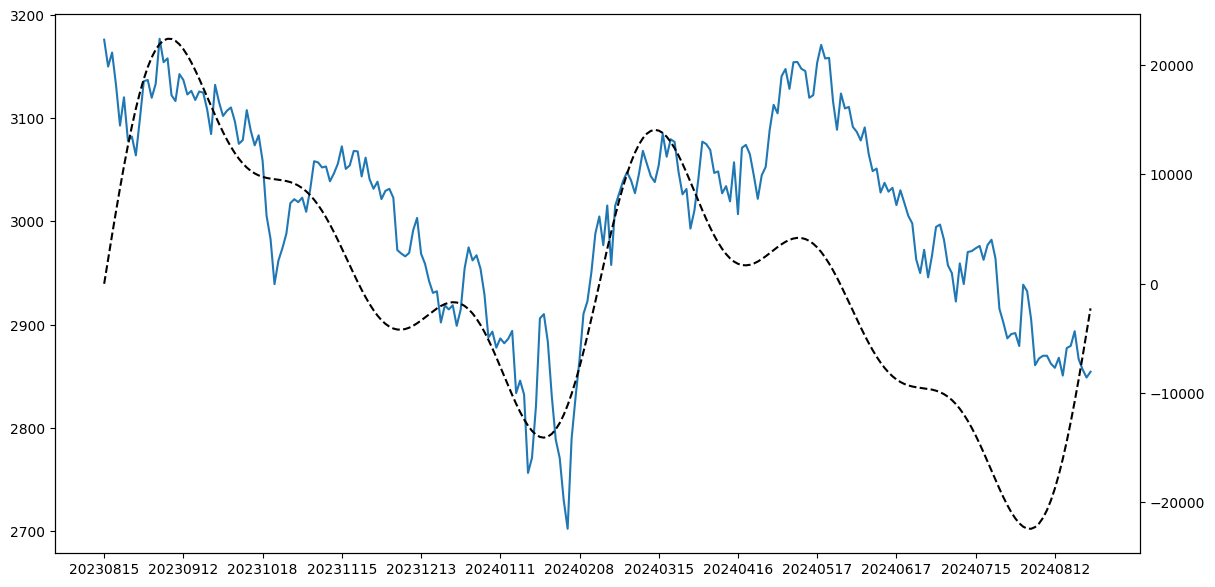
The major cycles basically match, meaning these capital flows basically control the market trend. Moreover, we seem to be able to assert that during the period from March 15 to May 17, there was a divergence trend between stock prices and main force capital: main force capital was retreating, but retail investors were still operating. Thus, although stock prices were still rising, the final direction was determined by main force capital.
tip
The black line is synthesized from the main force capital waves (predictive for the future). Before the market undergoes fundamental changes, the main force's operational style is relatively fixed, so it may have some short-term predictive ability. If we accept this conclusion, we should note that there is another divergence at the end -- retail investors are still leaving, but main force capital is entering. Of course, please do not take this too seriously.I used to think that the DC component indicates the trend of asset prices, but in fact, all waves are horizontal -- but only commodity markets are horizontal, while stock markets are essentially upward. Therefore, the DC component cannot indicate the trend of asset prices.
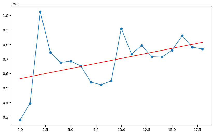
Until today, a sudden idea struck me: if you segment a longer time series signal and perform FFT decomposition, you will obtain several DC components. The regression line of these DC components is the trend of asset prices.
Here are three hypotheses:
If the energy distribution at various frequencies does not change significantly after segmented decomposition, it indicates that the composition of investors and their operational styles have not changed significantly. We can use FFT to predict short-term future trends until the conditions no longer hold.
The DC component of the Shanghai Composite Index over the past 30 years should be able to perfectly fit a trend line, and its slope equals the slope of the 20-year regression line of the Shanghai Composite Index.
Securities prices are a combination of the trend line of the DC component and a series of sine waves.
Next, we will prove the second hypothesis (process omitted). Finally, we plot the DC component and trend line as follows:
And the A-share annual lines and trend lines since 2005 are as follows:
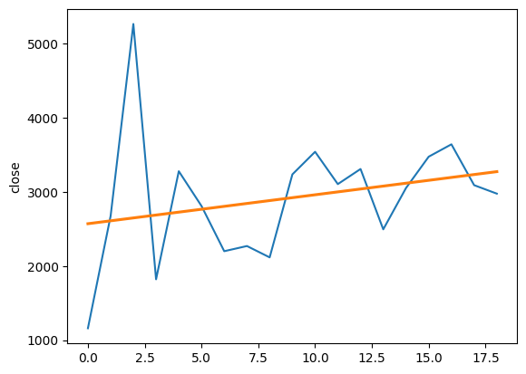
It cannot be said to be very similar, but almost completely consistent.
The p-value for trend line fitting is around 0.055, which basically meets the 0.05 confidence level requirement.
This article is part of our "Factor Investing and Machine Learning Strategies," appearing in the section on exploring new factor methodologies. Some important results obtained from FFT transformation will become features used to train machine learning strategies. See you in class for more content!
Essential NUMPY Programming for Quants (1) - Core Syntax
1. Basic Data Structures
The core data structure of NumPy is ndarray (n-dimensional array). This is an object representing multi-dimensional, homogeneous, and fixed-size arrays.
ndarray can only store homogeneous array objects, making it unable to express record-type data. Therefore, NumPy has extended to a data structure called structured array. It uses a void type tuple to represent a record, allowing NumPy to also express record-type data. Therefore, in NumPy, there are actually two main data types related to arrays.
The former array format is well-known, and we will use it as an example to introduce most NumPy operations. The latter data format is also commonly used in quantitative finance, such as market data obtained through Juheshi's [^Juheshi] jqdatasdk, which allows returning this type of data. Compared to DataFrame, it has many conveniences in storage and access. We will introduce it in a separate chapter later.
Before using NumPy, we must first install and import the NumPy library:
# 安装 NUMPY
pip install numpyGenerally, we import and use NumPy via the alias np:
import numpy as npTo make the results more prominent when running these examples in a Notebook, we first define a cprint function that outputs prompts as-is but uses red font for variables to distinguish them:
from termcolor import colored
def cprint(formatter: str, *args):
colorful = [colored(f"{item}", 'red') for item in args]
print(formatter.format(*colorful))
# 测试一下 CPRINT
cprint("这是提示信息,后接红色字体输出的变量值:{}", "hello!")Next, we will introduce basic add, delete, modify, and query operations.
1.1. Creating Arrays
1.1.1. Creating via Python List
We can create a simple array via the np.array syntax:
arr = np.array([1, 2, 3])
cprint("create a simple numpy array: {}", arr)In this syntax, we can provide a Python list or any object with an Iterable interface, such as a tuple.
1.1.2. Pre-set Special Arrays
Often, we hope NumPy will create arrays with special values. NumPy indeed provides such support, for example:
| Function | Description |
|---|---|
| zeros zeros_like |
Create an array of all 0s. zeros_like accepts another array and generates a zeros array of the same shape and data type. Commonly used for initialization. The following *_like functions are similar. |
| ones ones_like |
Create an array of all 1s. |
| full full_like |
Create an array where all elements are filled with n. |
| empty empty_like |
Create an empty array. |
| eye identity |
Create an identity matrix. |
| random.random | Create a random array. |
| random.normal | Create a random array following a normal distribution. |
| random.dirichlet | Create a random array following a Dirichlet distribution. |
| arange | Create an incrementing array. |
| linspace | Create a linearly growing array. The difference from arange is that this method generates a fully closed interval array by default. Also, the interval between its elements can be floating-point numbers. |
# 创建特殊类型的数组
cprint("全 0 数组:\n{}", np.zeros(3))
cprint("全 1 数组:\n{}", np.ones((2, 3)))
cprint("单位矩阵:\n{}", np.eye(3))
cprint("由数字 5 填充的矩阵:\n{}", np.full((3,2), 5))
cprint("空矩阵:\n{}", np.empty((2, 3)))
cprint("随机矩阵:\n{}",np.random.random(10))
cprint("正态分布的数组:\n{}",np.random.normal(10))
cprint("狄利克雷分布的数组:\n{}",np.random.dirichlet(np.ones(10)))
cprint("顺序增长的数组:\n{}", np.arange(10))
cprint("线性增长数组:\n{}", np.linspace(0, 2, 9))warning
Although the name of the `empty` function implies it should generate an empty array, the generated array actually has values for each element. These values are neither `np.nan` nor `None`, but random values. Before using an array generated by `empty`, we must initialize it and handle these random values.Generating normal distribution arrays is very useful. When conducting research, we often need to generate price sequences satisfying certain conditions to further study and compare their characteristics.
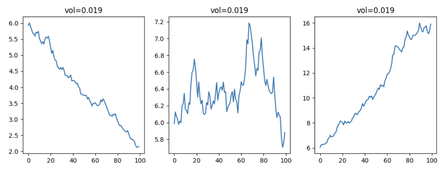
For example, if we want to study certain indicators under upward and downward trends, we need the ability to first construct price sequences that conform to trends. The following example demonstrates how to generate such sequences and plot them:
import numpy as np
import matplotlib.pyplot as plt
returns = np.random.normal(0, 0.02, size=100)
fig, axes = plt.subplots(1, 3, figsize=(12,4))
c0 = np.random.randint(5, 50)
for i, alpha in enumerate((-0.01, 0, 0.01)):
r = returns + alpha
close = np.cumprod(1 + r) * c0
axes[i].plot(close)The plotted graph is as follows:
The example also mentions Dirichlet distribution arrays. These arrays have the characteristic that the sum of all their elements equals 1. For example, in the efficient frontier optimization of modern portfolio theory, we first need to initialize the weights of various assets (random values) and satisfy the constraint that the sum of asset weights equals 1 (obviously!). At this point, we can use the Dirichlet[^Dirichlet] distribution.
info
Dirichlet, a German mathematician. He made outstanding contributions to number theory, Fourier series theory, and other fields of mathematical analysis and is considered one of the earliest mathematicians to give the modern definition of a function and one of the founders of analytic number theory.Note the role of axis in the concatenate function:
arr = np.arange(6).reshape((3,2))
# 在 ROW 方向上拼接,相当于增加行,默认行为
cprint("按 axis=0 拼接:\n{}", np.concatenate((arr, arr), axis=0))
# 在 COL 方向上拼接,相当于扩展列
cprint("按 axis=1 拼接:\n{}", np.concatenate((arr, arr), axis=1))1.2. Adding/Deleting and Modifying Elements
NumPy arrays are of fixed size, and we generally do not recommend frequently adding or deleting elements from arrays. But if there is indeed such a need, we can use the following methods to achieve adding or deleting:
| Function | Description |
|---|---|
| append | Add values to the end of arr. |
| insert | Insert value value (can be a scalar or an array) at the position specified by obj (can be an index, slicing). |
| delete | Delete elements at specified indices. |
Examples are as follows:
arr = np.arange(6).reshape((3,2))
np.append(arr, [[7,8]], axis=0)
cprint("指定在行的方向上操作、n{}", arr)
arr = np.arange(6).reshape((3,2))
arr = np.insert(arr.reshape((3,2)), 1, -10)
cprint("不指定 axis,数组被扁平化:\n{}", arr)
arr = np.arange(6).reshape((3,2))
arr = np.insert(arr, 1, (-10, -10), axis=0)
cprint("np.insert:\n{}", arr)
arr = np.delete(arr, [1], axis=1)
cprint("deleting col 1:\n{}", arr)tip
Please definitely run the code here, especially the part about `insert`, to understand what flattening means.Sometimes we need to modify the values of individual elements. We should operate as follows:
arr = np.arange(6).reshape(2,3)
arr[0,2] = 3This involves how to locate an array element, which is the content of our next section.
1.3. Locating, Reading, and Searching
1.3.1. Indexing and Slicing
The indexing and slicing syntax in NumPy is roughly similar to Python, with the main difference being support for multi-dimensional arrays:
arr = np.arange(6).reshape((3,2))
cprint("原始数组:\n{}", arr)
# 切片语法
cprint("按行切片:{}", arr[1, :])
cprint("按列切片:{}", arr[:, -1])
cprint("逆排数组:\n {}", arr[: : -1])
# FANCY INDEXING
cprint("fancy index: 使用下标数组:\n {}", arr[[2, 1, 0]])
The above slicing syntax also exists in Python, but it only supports up to one dimension. Therefore, for the following Python array, similar operations will fail:
arr = np.arange(6).reshape((3,2)).tolist()
arr[1, :]Prompt: list indices must be integers or slices, not tuple.
1.3.2. Finding, Filtering, and Replacing
In the previous section, we located an array element via indexing. But often, we first need to find the indices that meet the requirements through conditional operations. This section will introduce related methods.
| Function | Description |
|---|---|
| np.searchsorted | Search for specified values in an ordered array and return the index. |
| np.nonzero | Return the indices of non-zero elements, used to find elements in the array that meet the conditions. |
| np.flatnonzero | Same as nonzero, but returns the indices of non-zero elements in the flattened version of the input array. |
| np.argwhere | Return the indices of elements that meet the conditions, equivalent to the transpose version of nonzero. |
| np.argmin | Return the index of the smallest element in the array (note: not the smallest index that meets the conditions). |
| np.argmax | Return the index of the largest element in the array. |
# 查找
arr = [0, 2, 2, 2, 3]
pos = np.searchsorted(arr, 2, 'right')
cprint("在数组 {} 中寻找等于 2 的位置,返回 {}, 数值是 {}",
arr, pos, arr[pos - 1])
arr = np.arange(6).reshape((2, 3))
cprint("arr[arr > 1]: {}", arr[arr > 1])
# NONZERO 的用法
mask = np.nonzero(arr > 1)
cprint("nonzero 返回结果是:{}", mask)
cprint("筛选后的数组是:{}", arr[mask])
# ARGWHERE 的用法
mask = np.argwhere(arr > 1)
cprint("argwere 返回的结果是:{}", mask)# 多维数组不能直接使用 ARGWHERE 结果来筛选
# 下面的语句不能得到正确结果,一般会出现 INDEXERROR
arr[mask]
# 但对一维数组筛选我们可以用:
arr = np.arange(6)
mask = np.argwhere(arr > 1)
arr[mask.flatten()[0]]
# 寻找最大值的索引
arr = [1, 2, 2, 1, 0]
cprint("最大值索引是:{}", np.argmax(arr))When using searchsorted, note that the array itself must be ordered; otherwise, it will not yield correct results.
Lines 10 to 21 show how to find data in an array that meets the conditions and return its index.
The return value of argwhere is equivalent to the transpose of nonzero. In the case of multi-dimensional arrays, it cannot be directly used as an array index. Please compare the usage of nonzero and argwhere yourself.
In quantitative finance, there are many situations requiring filtering functionality. For example, when calculating upper and lower shadows, we use the formula $(high - max(open, close))/(high - low)$ for calculation. If we want to calculate the upper shadows for the past $n$ periods all at once without using loops, we must use filtering functions like np.where and np.select.
The following example shows how to use np.select to calculate upper shadows:
import pandas as pd
import numpy as np
bars = pd.DataFrame({
"open": [10, 10.2, 10.1],
"high": [11, 10.5, 9.3],
"low": [9.8, 9.8, 9.25],
"close": [10.1, 10.2, 10.05]
})max_oc = np.select([bars.close > bars.open,
bars.close <= bars.open],
[bars.close, bars.open])
print(max_oc)
shadow = (bars.high - max_oc)/(bars.high - bars.low)
print(shadow)
np.where is a function similar to np.select, but it only accepts one condition.
arr = np.arange(6)
cprint("np.where: {}", np.where(arr > 3, 3, arr))This code implements the function of clipping numbers above 3 to 3. This function is called clip, a very common technique in factor preprocessing used to handle outliers.
But it cannot achieve clipping at both ends. At this point, np.select can do it, which is the main difference between np.where and np.select:
arr = np.arange(6)
cprint("np.select: {}", np.select([arr<2, arr>4], [2, 4], arr))The result is that in the generated array, values less than 2 are replaced with 2, values greater than 4 are replaced with 4, and others remain unchanged.
1.4. Inspecting Arrays
When calling other people's libraries, we often need to exchange data with them. At this time, there may be data format incompatibility issues. To be able to troubleshoot, we must master some methods for viewing the characteristics of NumPy arrays.
We first generate a simple array as follows, and then view its various characteristics:
arr = np.ones((3,2))
cprint("dtype is: {}", arr.dtype)
cprint("shape is: {}", arr.shape)
cprint("ndim is: {}", arr.ndim)cprint("size is: {}", arr.size)
cprint("'len' is also available: {}", len(arr))
# DTYPE
dt = np.dtype('>i4')
cprint("byteorder is: {}", dt.byteorder)
cprint("name of the type is: {}", dt.name)
cprint('is ">i4" a np.int32?: {}', dt.type is np.int32)
# 复杂的 DTYPE
complex = np.dtype([('name', 'U8'), ('score', 'f4')])
arr = np.array([('Aaron', 85), ('Zoe', 90)], dtype=complex)
cprint("A structured Array: {}", arr)
cprint("Dtype of structured array: {}", arr.dtype)Just as Python objects have their own data types, NumPy arrays also have their own data types. We can view the data type of the array via arr.dtype.
From line 3 to line 6, we output the array's shape, ndim, size, and len attributes, respectively. ndim tells us the dimension of the array. shape tells us the size of each dimension. shape itself is a tuple, and the size of this tuple equals ndim.
size returns the product of the values of each element in shape when no parameters are passed. len returns the length of the first dimension.
1.5. Array Operations
We have already seen some examples in the previous sections that cause changes in array shape. For example, to generate a $3×2$ array, we first use np.arange(6) to generate a one-dimensional array, and then change its shape to (2, 3).
Another example is using np.concatenate, which changes the rows or columns of the array.
1.5.1. Dimension Increasing
We can change the dimension of the array via reshape, hstack, vstack:
cprint("increase ndim with reshape:\n{}",
np.arange(6).reshape((3,2)))
# 将两个一维数组,堆叠为 2*3 的二维数组
cprint("createing from stack: {}",
np.vstack((np.arange(3), np.arange(4,7))))
# 将两个 (3,1)数组,堆叠为(3,2)数组
np.hstack((np.array([[1],[2],[3]]), np.array([[4], [5], [6]])))1.5.2. Dimension Decreasing
Perform dimension reduction on the array via ravel, flatten, reshape, *split operations.
cprint("ravel: {}", arr.ravel())
cprint("flatten: {}", arr.flatten())
# RESHAPE 也可以用做扁平化
cprint("flatten by reshape: {}", arr.reshape(-1,))
# 使用 HSPLIT, VSPLIT 进行降维
x = np.arange(6).reshape((3, 2))
cprint("split:\n{}", np.hsplit(x, 2))
# RAVEL 与 FLATTEN 的区别:RAVEL 可以操作 PYTHON 的 LIST
np.ravel([[1,2,3],[4, 5, 6]])This introduces a total of 4 methods. ravel and flatten have similar usage. The behavior of ravel is similar to flatten, except that ravel is a function of np and can act on ArrayLike arrays.
Flattening via reshape is also a common operation. Additionally, vsplit and hsplit functions are introduced, whose functions are exactly opposite to vstack and hstack.
1.5.3. Transposition
Additionally, transposing the array is also one such example.
For example, earlier we mentioned that the result of np.argwhere is actually the transpose of np.nonzero. Let's verify this:
x = np.arange(6).reshape(2,3)
cprint("argwhere: {}", np.argwhere(x > 1))
# 我们再来看 NP.NONZERO 的转置
cprint("nonzero: {}", np.array(np.nonzero(x > 1)).T)The two output results are exactly the same. Here, we achieved transposition via .T, which is a syntax sugar. The formal function is transpose.
Of course, due to the extreme power of the reshape function, we can also use it to complete transposition:
cprint("transposing array from \n{} to \n{}",
np.arange(6).reshape((2,3)),
np.arange(6).reshape((3,2)))