QuanTide Weekly: Macro Signals, Factor Papers, and NumPy Core
This Week’s Highlights
- PBOC: Room for Reserve Requirement Ratio (RRR) cuts, but further rate declines face constraints
- Buffett trims Bank of America again—shorting his own country?
- Expectations for existing mortgage rate cuts dashed; CSI 300 closes below 2800 for three consecutive days
Next Week’s Watchlist
- Monday: August CPI/PPI data release
- Monday: Kweichow Moutian earnings briefing; its outlook on the baijiu sector is a key signal
This Week’s Selections
- Must-Read Quantitative Finance Papers
- Series: Essential Numpy Programming for Quants (Part 2)
This Week’s Highlights
- On September 5, Zou Lan from the PBOC’s Monetary Policy Department stated that whether to cut the RRR or interest rates depends on economic trends. The policy effects of the RRR cut earlier this year are still materializing. Currently, the average statutory deposit reserve ratio for financial institutions is approximately 7%, leaving room for further cuts. However, factors such as the pace of deposit migration to asset management products and the narrowing of banks’ net interest margins impose constraints on further declines in deposit and lending rates.
- On September 5 (local time), the U.S. Securities and Exchange Commission disclosed that Warren Buffett reduced his holdings in Bank of America over three consecutive days around September 4, cashing out approximately $760 million. In July, he had sold Bank of America shares for nine consecutive days. Before these reductions, Bank of America was his second-largest position and one of Berkshire Hathaway’s most profitable companies.
- The Shanghai Composite Index fell 2.69% this week, closing below 2800 for three consecutive days. The index’s P/E ratio is currently at the 12th percentile, a relatively low level. On the news front, last week’s widely rumored rate cuts for existing mortgages failed to materialize.
- New regulations on listed company pre-IPO shareholding by former CSRC employees have taken effect, imposing stricter requirements and broader verification scopes.
Must-Read Quantitative Finance Papers
- Portfolio Selection, Markowitz, 1952. In this paper, Markowitz proposed Modern Portfolio Theory (MPT), for which he received the 1990 Nobel Prize in Economics. The paper extended the common risk-return trade-off by incorporating the correlation between risk and return into calculations.
- A New Interpretation of Information Rate, Kelly, 1956. This paper presents the formal statement of the famous Kelly Criterion. The model is widely used in casino games, particularly in risk management. The author derived a formula that determines the optimal allocation size to maximize wealth growth over time.
- Capital Asset Prices: A Theory of Market Equilibrium under Conditions of Risk (Sharpe, 1964). Building on Markowitz’s work, CAPM demonstrated that there is only one efficient portfolio: the market portfolio. This paper introduced the famous Beta concept. Sharpe and Markowitz were teacher and student, respectively, and both received the Nobel Prize in Economics in the same year.
- Efficient Capital Markets: a Review of Theory and Empirical Work, Fama, 1970. This paper is the seminal work that first proposed the highly popular "Efficient Market Hypothesis." Although this theory is now heavily questioned, its academic value remains high.
- The Pricing of Options and Corporate Liabilities, Black & Scholes, 1973. The famous BS formula uses the heat transfer equation from physics as a starting point for estimating option prices. This is also why hedge funds favor physics graduates.
- Does the Stock Market Overreact?, Bondt & Thaler, 1985. This paper challenges the Efficient Market Hypothesis. Bondt and Thaler present statistically significant evidence to the contrary, suggesting that investors often overreact to unexpected news events. This is one of the classic studies in behavioral finance, which has been a major theme for Nobel Prizes in recent years. Its underlying philosophy is subjective value theory and human-centric thinking. Thaler, a Nobel laureate, even played himself in the movie The Big Short.
- A closed-form GARCH option valuation model, Heston & Nandi, 1997. This paper proposes a closed-form formula for valuing spot assets and models their variance using a Generalized Autoregressive Conditional Heteroskedasticity (GARCH) model. Due to its complexity and practicality, GARCH models were widely popular for estimating volatility in the 1990s and were actively adopted by the financial industry.
- Optimal Execution of Portfolio Transactions, Almgren & Chriss, 2000. For any quant developer responsible for refining trade execution algorithms, this paper is an absolute must-read. The paper points out that price volatility stems from exogenous factors (market volatility) and endogenous factors (the impact of one’s own orders on the market). This is a quantum effect! The authors formalized a method for executing and measuring trade execution performance by minimizing a combination of transaction costs and volatility risk.
- Incorporating Signals into Optimal Trading, Lehalle, 2017. Very similar to the work of Almgren and Chriss (2000), this paper discusses optimal trade execution. The authors further refined the work in this field by incorporating Markov signals into the optimal trading framework and derived optimal trading strategies for the special case of assets with drift (Ornstein-Uhlenbeck processes).
- The Performance of Mutual Funds in the Period 1945-1964, Michael Jessen. Sharpe introduced the concept of Beta in his paper, while the concept of Alpha was introduced by Jessen in this paper.
- Common risk factors in the returns on stocks and bonds, Fama, 1993. In this paper, Fama proposed the three-factor model.
- Review of Financial Studies, Stambaugh & Yuan, 2017. This paper was published relatively late, allowing it to review important papers on factor investing that appeared earlier, making it an essential read for quickly understanding the industry. Despite its late publication, it has garnered 952 citations.
- 151 Trading Strategies, Kakushadze, 2018. The author is from WorldQuant and is one of the authors of Alpha101. This paper cites a large number of other papers (2000+), making it excellent material for broad reading.
Essential NumPy Programming for Quants (Part 2) - Core Syntax
1. Structured Arrays
Initially, NumPy arrays could only store homogeneous elements, meaning all elements had to share the same data type. However, many tabular data sets consist of records, where each record is composed of data with different data types. For example, in the most common market data, it must include at least time, security codes, and OHLC (Open, High, Low, Close) data.
To meet this need, NumPy introduced a data format called Structured Arrays. It is a one-dimensional array where each element is a named tuple.
We can declare a Structured Array as follows:
import numpy as np
import datetime
dtypes = [
("frame", "O"),
("code", "O"),
("open", "f4"),
("high", "f4"),
("low", "f4"),
("close", "f4")
]
secs = np.array(
[
(datetime.date(2024, 3, 18), "600000", 8.9, 9.1, 8.8, 9),
(datetime.date(2024, 3, 19), "600000", 8.9, 9.1, 8.8, 9),
], dtype = dtypes
)In this data structure, there are six fields, with their names and types defined via dtype. This is a List[Tuple] type. In the data initialization section, it is also a List[Tuple].
warning
A common mistake for beginners is using `List[List]` to initialize a NumPy Structured Array instead of `List[Tuple]`. This causes NumPy to fail to match the correct data type during array construction, resulting in strange errors.For example, the following initialization is incorrect:
secs = np.array([
[datetime.date(2024, 3, 18), "600000", 8.9, 9.1, 8.8, 9],
[datetime.date(2024, 3, 19), "600000", 8.9, 9.1, 8.8, 9]
], dtype=dtypes)This code will report an obscure "Type Error: float() argument must be a string or ..."
print(f"secs的维度是{secs.ndim}")
print(f"secs的shape是{secs.shape}")
print(f"secs的size是{secs.size}")
print(f"secs的length是{len(secs)}")
print(f"secs[0]的类型是{type(secs[0])}")
print(f"secs[0]的维度是{secs[0].ndim}")
print(f"secs[0]的shape是{secs[0].shape}")
print(f"secs[0]的size是{secs[0].size}")
print(f"secs[0]的length是{len(secs[0])}")As shown, the secs array is a one-dimensional array, and its shape (2,) correctly represents the shape of a 1D array. The previous section also introduced the relationships between these attributes; you can verify if they still hold.
However, the element type of secs is numpy.void, which is essentially a named tuple. Therefore, we can access any field as follows:
print(secs[0]["frame"])
# 不使用列名(字段名),使用其序号也是可以的
print(secs[0][0])We can also access a "cell" in column-major order:
print(secs["frame"][0])For tabular data, iteration is a common operation. We can iterate as follows:
for (frame, code, opn, high, low, close) in secs:
print(frame, code, opn, high, low, close)NumPy structured arrays are much more user-friendly in this aspect than Pandas DataFrames. We will mention this again when introducing Pandas later.
2. Arithmetic Operations
2.1. Comparison and Logical Operations
In the previous section on locating and searching, we encountered comparisons, such as arr > 1. This compares every element in the array with 1 and returns a boolean array.
Now, we expand the comparison instructions:
| Function | Description |
|---|---|
| all | Returns True if all elements in the array are true. Used to check if a set of conditions holds simultaneously. |
| any | Returns True if at least one element in the array is true. Used to check if at least one condition holds. |
| isclose | Checks if elements in two arrays are approximately equal one-by-one, returning all comparison results. |
| allclose | Checks if all elements in two arrays are approximately equal. |
| equal | Checks if elements in two arrays are equal one-by-one, returning all comparison results. |
| not_equal | Checks if elements in two arrays are unequal one-by-one, returning all comparison results. |
| isfinite | Checks if the value is a number and not infinite. |
| isnan | Tests if the value is Not a Number. |
| isnat | Tests if the object is not of time type. |
| isneginf | Tests if the object is negative infinity. |
| isposinf | Tests if the object is positive infinity. |
# 开启多行输出模式
from IPython.core.interactiveshell import InteractiveShell
InteractiveShell.ast_node_interactivity = "all"
np.random.seed(78)
returns = np.random.normal(0, 0.03, size=4)
returns
# 判断是否全下跌
np.all(returns <= 0)
np.any(returns <= 0)
# 模拟一个起始价格为8元的价格序列
prices = np.cumprod(1+returns) * 8
# 对应的涨停价如下
buy_limit_prices = [8.03, 8.1, 8.1, 8.3]
# 判断是否涨停
np.isclose(prices, buy_limit_prices, atol=1e-2)In addition to checking if all elements in an array are True or if at least one is True, we sometimes need fuzzy judgments. For example, if more than 60% of the past 20 days show bullish candles, we can use np.count_nonzero or np.sum to count the number of True values in the array:
np.count_nonzero(returns > 0)
np.sum(returns > 0)In the previous section’s comparison examples, we only used single conditions. If we need to search based on a combination of multiple conditions, we must rely on logical operations.
In NumPy, logical operations can be performed via functions or operators:
| Function | Operator | Description | Python Equivalent |
|---|---|---|---|
| logical_and | & | Performs logical AND | and |
| logical_or | | | Performs logical OR | or |
| logical_not | ~ | Performs logical NOT | not |
| logical_xor | '^' | Performs logical XOR | xor |
What is the use of logical operations? For example, in stock selection, we have the following tabular data:
| Stock | PE | MOM |
|---|---|---|
| AAPL | 30.5 | 0.1 |
| GOOG | 32.3 | 0.3 |
| TSLA | 900.1 | 0.5 |
| MSFT | 35.6 | 0.05 |
The above table can be represented in NumPy using a Structured Array:
tickers = np.array([
("APPL", 30.5, 0.1),
("GOOG", 32.3, 0.3),
("TSLA", 900.1, 0.5),
("MSFT", 35.6, 0.05)
], dtype=[("ticker", "O"), ("pe", "f4"), ("mom", "f4")])Now, we want to find records where PE < 35 and Momentum (MOM) > 0.2. We can construct the condition expression as follows:
(tickers["pe"] < 35) & (tickers["mom"] > 0.2)NumPy will compare all values in the PE column with 35, then perform a logical AND operation with the results of comparing MOM with 0.2, which is equivalent to:
np.array((1,1,0,0)) & np.array((0, 1, 1, 0))In NumPy, True is equal to 1 in logical operations, and 0 is equal to False.
Without NumPy’s logical operations, we would have to use Python’s logical operations, which unfortunately require loops. If the computational load is large, this will be time-consuming.
Examples of using XOR in quantitative finance are most likely found in stock selection. For instance, if we require that we only buy when exactly one of two selection conditions is met (and do not buy otherwise), we can use the XOR operation.
2.2. Set Operations
In trading, we often need to perform rebalancing. The general approach is to determine the new portfolio, compare it with the current portfolio, and identify stocks to sell and stocks to buy. This operation is a set operation. In Python, we typically use set syntax to implement this.
In NumPy, we can implement set operations using the following methods:
import numpy as np
# 创建两个一维数组
x = np.array([1, 2, 3, 4, 5])
y = np.array([4, 5, 6, 7, 8])
# 计算交集
intersection = np.intersect1d(x, y)
print("Intersection (交集):", intersection)
# 计算并集
union = np.union1d(x, y)
print("Union (并集):", union)diff = np.setdiff1d(x, y)
print("x - y:", diff)Additionally, we might use the in1d(a1, a2) method to determine if all elements in a1 exist in a2. For example, in portfolio rebalancing, if the current holdings are all included in the buy plan, no rebalancing is needed.
2.3. Mathematical and Statistical Operations
Mathematical operations in NumPy include linear algebra operations (as well as basic algebraic operations), statistical operations, and financial indicator calculations.
2.3.1. Linear Algebra
Linear algebra has important applications in quantitative finance. For example, in Modern Portfolio Theory (MPT), we need to calculate portfolio returns and covariances, which require matrix multiplication. You can refer to the Portfolio Theory and Practice series for reference. Below is a snippet of code:
...
cov = np.cov(port_returns.T)
port_vol = np.sqrt(np.dot(np.dot(weights, cov), weights.T))Matrix multiplication is a core concept in linear algebra. It involves multiplying specific elements of two matrices according to rules and summing them to generate a new matrix. Specifically, if matrix A is of dimension $m \times n$ and matrix B is of dimension $n \times p$, their product $C = AB$ will be a matrix of dimension $m \times p$. The rule of multiplication is that each element of a row in A is multiplied by the corresponding element of a column in B, and the results are summed.
The following example illustrates the process of matrix multiplication:
Assume we have two matrices A and B:
$$ A = \begin{bmatrix} 2 & 3 \ 1 & 4 \ \end{bmatrix} $$ and $$ B = \begin{bmatrix} 1 & 2 \ 3 & 1 \ \end{bmatrix} $$ To calculate AB, we follow these steps:
Take the first row of A $(2, 3)$ and the first column of B $(1, 3)$, multiply corresponding elements, and sum them to get $C_{11} = [2\times1 + 3\times3 = 11]$.
Similarly, take the first row of A and the second column of B $(2, 1)$, multiply corresponding elements, and sum them to get $C_{12} = [2\times2 + 3\times1 = 7]$.
Take the second row of A $(1, 4)$ and the first column of B, multiply corresponding elements, and sum them to get $C_{21} = [1\times1 + 4\times3 = 13]$.
Take the second row of A and the second column of B, multiply corresponding elements, and sum them to get $C_{22} = [1\times2 + 4\times1 = 5]$.
Therefore, matrix C = AB is:
$$ C = \begin{bmatrix} 11 & 7 \ 13 & 6 \ \end{bmatrix} $$
Unlike algebraic operations, matrix multiplication does not satisfy the commutative law, i.e., generally $AB \neq BA$.
In NumPy, we can use the np.dot() function to calculate matrix multiplication.
The above example expressed in NumPy is:
A = np.array([[2,3],[1,4]])
B = np.array([[1,2],[3,1]])
np.dot(A, B)Ultimately, we will obtain the same result as matrix C.
In addition, matrix inversion (np.linalg.inv) is used to solve systems of equations when calculating optimal portfolio weights, while eigenvalues and eigenvectors (np.linalg.eig, np.linalg.svd) are used in analyzing principal components of asset returns and performing risk decomposition.
2.3.2. Statistical Operations
Common statistical operations include:
| Function | Description |
|---|---|
| np.mean | Calculate the mean |
| np.median | Calculate the median |
| np.std | Calculate the standard deviation |
| np.var | Calculate the variance |
| np.min | Calculate the minimum value |
| np.max | Calculate the maximum value |
| np.percentile | Calculate quantiles of historical data |
| np.quantile | Calculate quantiles of historical data; same function as percentile |
| np.corr | Calculate correlation between two variables |
np.percentile and np.quantile have the same function, both used for calculating quantiles. They differ slightly in parameters.
When applying them to the same array, passing a quantile point of 0.25 to quantile yields the same result as passing 25 to percentile, meaning the latter is multiplied by 100. In quantitative trading, quantile is used more frequently.
A common application of np.percentile (or np.quantile) is calculating the 25%, 50%, and 75% quantiles to draw box plots (Boxplots).
Additionally, we often use it to select adaptive parameters. For example, in RSI applications, it is generally recommended to buy when below 20 (or 30) as oversold, and sell when above 80 (or 70) as overbought. However, with some statistical analysis, you will find that these thresholds are not fixed. If we use the RSI over a past period for statistics, using its 95% quantile as the sell point and 15% as the buy point often yields better results.
2.3.3. Calculation of Quantitative Indicators
Some common quantitative indicator calculations can also be performed using NumPy. For example, calculating moving averages can be done using NumPy’s convolve function.
import numpy as np
def moving_average(data, window_size):
return np.convolve(data, np.ones(window_size)/window_size, 'valid')Of course, many people are accustomed to using talib or Pandas’ rolling function for calculations. convolve (convolution) is the core of neural networks (CNNs), which is why we mention it here.
The second parameter of np.convolve is the convolution kernel. Here, we are implementing a Simple Moving Average (SMA), so the convolution kernel is an array of identical values. Its length is the window size, and the sum of its elements is 1.
If we replace the convolution kernel with other values, we can implement indicators like WMA (Weighted Moving Average). From a signal processing perspective, moving average is a form of signal smoothing. Using different convolution kernels achieves different smoothing effects.
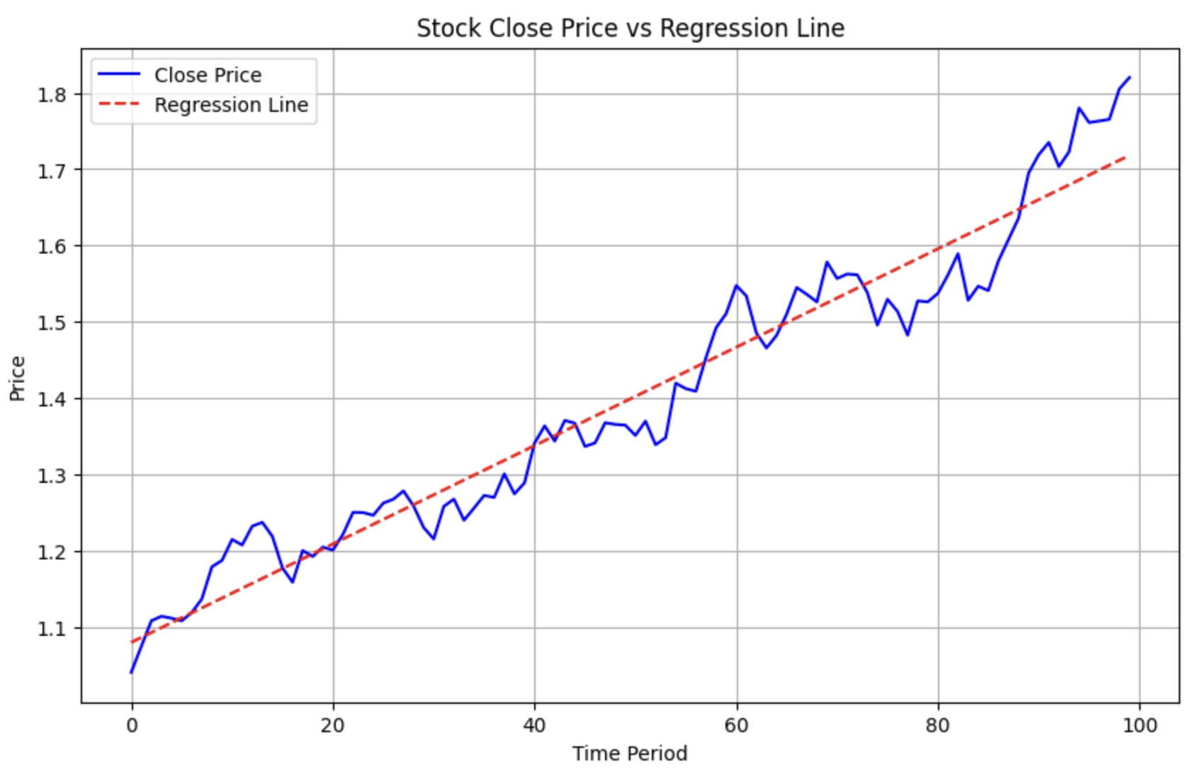
In quantitative finance, another type of calculation worth mentioning is polynomial regression. For example, if two stocks have recently shown an upward trend, and we want to know which one is performing better, we can perform polynomial regression, fit them to a straight line, and then compare their slopes.
The following code demonstrates how to perform polynomial regression using NumPy.
import numpy as np
import matplotlib.pyplot as plt
returns = np.random.normal(0, 0.02, size=100)
alpha = 0.01
close = np.cumprod(1 + returns + alpha)
a, b = np.polyfit(np.arange(100), close, deg=1)
# 继续之前的代码
# 使用a, b构建回归线的y值
regression_line = a * np.arange(100) + b
# 绘制原始的close曲线
plt.figure(figsize=(10, 6))
plt.plot(close, label='Close Price', color='blue')
# 绘制回归线
plt.plot(regression_line, label='Regression Line', color='red', linestyle='--')
# 添加图例、标题和坐标轴标签
plt.title('Stock Close Price vs Regression Line')
plt.xlabel('Time Period')
plt.ylabel('Price')
plt.legend()
# 显示图表
plt.grid(True)
plt.show()This will generate the following image:
Python 3.10+ Type Hints & NumPy Type Conversion
Mastering NumPy type conversion and Python 3.10+ type hints for robust quantitative factor investing and machine learning pipelines.
3. Type Conversion and Typing
When exchanging data between different libraries, format mismatches are common. For instance, market data from third-party sources often uses strings for timestamp fields (a result of skipping a few lines of code?). Some libraries optimize storage for OHLC fields using 4-byte floats, but if you need to pass this data to talib for indicator calculations, you must first convert it to 8-byte floats. This creates a need for type conversion.
Additionally, we often need to convert NumPy data types to Python built-in types, such as converting numpy.float64 to float.
3.1. Internal NumPy Type Conversion
For internal NumPy type conversion, we simply use the astype function.
x = np.array(['2023-04-01', '2023-04-02', '2023-04-03'])
print(x.astype(dtype='datetime64[D]'))
x = np.array(['2014', '2015'])
print(x.astype(np.int32))
x = np.array([2014, 2015])
print(x.astype(np.str_))tips
How to convert a boolean array to an integer type, specifically converting `True` to `1` and `False` to `-1`? In calculations involving candlestick patterns (yang/yin lines), we often need to convert conditions like `open > close` into symbolic `1` and `-1` for subsequent calculations. This conversion can be achieved with:>>> x = np.array([True, False])
>>> x * 2 - 1
... array([ 1, -1])If we need to convert a NumPy array to a Python list, we can use the tolist function.
x = np.array([1, 2, 3])
print(x.tolist())We use the item() function to convert elements within a NumPy array into Python built-in types.
x = np.array(['2023-04-01', '2023-04-02'])
y = x.astype('M8[s]')
y[0].item()warning
An easily overlooked fact is that when extracting a scalar from a NumPy array, we should always convert it to a Python object before using it. Otherwise, hidden errors may occur, as shown in the following example:import json
x = np.arange(5)
print(json.dumps([0]))
print(x[0])
json.dumps([x[0]])The last line will fail with the error type int64 is not JSON serializable. Changing the last line to json.dumps([x[0].item()]) allows it to execute normally.
Starting from Python 3.1, type annotations (type hints) were introduced. By Python 3.8, a complete type annotation system was largely established. We often see parameter type annotations in functions, such as in the following code:
from typing import List
def add(a: List[int], b: int) -> List[int]:
return [i + b for i in a]This brings static type checking support to Python code.
The NumPy.typing module provides a series of type aliases and protocols, enabling developers to express NumPy array type information more precisely in type annotations. This helps static analysis tools, IDEs, and type checkers provide more accurate code completion, type checking, and error hints.
The main types provided by this module are ArrayLike, NDArray, and DType.
import numpy
from numpy.typing import ArrayLike, NDArray, DTypeLike
import numpy as np
def calculate_mean(data: ArrayLike) -> float:
"""计算输入数据的平均值,数据可以是任何ArrayLike类型"""
return np.mean(data)
def add_one_to_array(arr: NDArray[np.float64]) -> NDArray[np.float64]:
"""向一个浮点数数组的每个元素加1,要求输入和输出都是np.float64类型的数组"""
return arr + 1
def convert_to_int(arr: NDArray, dtype: DTypeLike) -> NDArray:
"""将数组转换为指定的数据类型"""
return arr.astype(dtype)If you are using the above functions in an IDE like VS Code, you can see the type hints for the functions. If the passed parameter type is incorrect, you will receive error hints during editing.
4. Further Reading
4.1. NumPy Data Types
In NumPy, the following common data types exist. Each numeric type has an alias. In places where a dtype parameter is required, either can generally be used. Additionally, aliases are better supported for string types and time/date types. For example, 'S5' is an alias for an ASCII string, but besides specifying the data type, it also specifies the string length. datetime64[S] indicates that the data is a date/time type, with precision down to seconds.
| Type | Alias | Category | Alias |
|---|---|---|---|
| np.int8 | i1 | np.float16 | f2 |
| np.int16 | i2 | np.float32 | f4, can also specify endianness, e.g., '<f4' for little-endian, '=' for native, '>f4' for big-endian. Other float types follow the same convention. |
| np.int32 | i4 | np.float64 | f8 |
| np.int64 | i8 | np.float128 | f16 |
| np.uint8 | u1 | np.bool_ | b1 |
| np.uint16 | u2 | np.str_ | U (followed by length, e.g., U10) |
| np.uint32 | u4 | np.bytes_ | S (followed by length, e.g., S5) |
| np.uint64 | u8 | np.datetime64 | |
| np.timedelta64 | m8 and m8[D] m8[h] m8[m] m8[s], etc. |
"Factor Investing and Machine Learning Strategies" Course is Now Open!

Live Online Stream on September 8th, Be There or Be Square