Weekly Highlights

• Market surge! The Shanghai Composite Index rose 12.8% this week, while the CSI 300 gained 15.7%.
• The first market-cap management guideline has been released, clarifying requirements for index constituents and stocks trading below book value.
• Changjiang Securities: Sectors such as banking, real estate, construction, and non-bank financials are more likely to benefit from the valuation enhancement plan for stocks trading below book value.

Next Week’s Outlook

• Monday: Caixin releases September PMI data.
• OpenAI hosts its 2024 annual DevDay event starting October 1.
• Market closed from Tuesday (October 1) to October 7.

Weekly Selection

• Series! Numpy Programming Essentials for Quants (Part 5)

• China A-shares surged across the board. On the news front, the State Council Information Office held a press conference on Tuesday to introduce financial support for high-quality economic development. Pre-market reserve requirement ratio (RRR) cuts and reductions in existing mortgage rates boosted market confidence. During trading, the capital market released a series of major positive developments: the CSRC is formulating the "M&A Six Measures," creating a 300 billion yuan stock repurchase and increase loan facility, launching a 50 billion yuan securities, fund, and insurance company swap facility, supporting long-term capital from entities like China Investment Corporation (CIC) to enter the market, and studying the creation of a stabilization fund.

Source: Eastmoney

• Caixin (September 28): Recently, the first market-cap management guideline for A-shares was released, clarifying specific requirements for index constituents and stocks trading below book value. Industry insiders stated that the new policy helps reprice undervalued high-quality assets, particularly state-owned enterprises (SOEs) with deep discounts to book value but stable profitability, potentially offering value revaluation opportunities and investment prospects. Another analyst noted that stocks trading below book value while offering high dividend yields deserve special attention from investors.
• The People’s Bank of China (PBOC) adjusted the 7-day reverse repo rate to 1.5%. This week, the PBOC also cut the reserve requirement ratio (RRR) by 0.5%.

Source: Caixin

Numpy Quantitative Application Case [2]

Momentum and mean reversion are the most critical quantitative factors. While there are many algorithms to characterize momentum, the slope of a fitted line is undoubtedly the most intuitive.

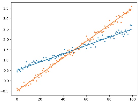
In the graph above, if the two lines represent the moving average trends of two stocks, you would obviously prefer to buy the orange one because it has a steeper slope, indicating faster growth.

Human vision has a powerful pattern-recognition capability. We can easily see that the upward trend of the orange points is stronger. However, to enable a computer to determine which dataset is better, we must fit a line, identify the trend line, and compare the slopes of the trend lines. Line fitting, curve fitting, or polynomial fitting are all linear regression problems.

In this chapter, we will discuss methods for line fitting, progressing from the most basic implementation to a vectorized implementation that is 100 times faster.

Linear Regression and Least Squares

How do we discover the hidden line that best reflects the trend among a set of random numbers? This problem has puzzled scientists since the Age of Discovery.

During that era, sailors needed to determine their latitude using celestial observations (longitude was calculated using solar eclipses), which required accurately describing celestial behavior based on human observations.

In addressing errors caused by celestial observations, French mathematician Adrien Marie Legendre first discovered the least squares method (1805). Later, Carl Friedrich Gauss proposed this method in his 1809 work Theoria Motus Corporum Coelestium. Ultimately, in 1829, he provided the theoretical proof that least squares is the best fit for linear regression. This proof is known as the Gauss-Markov theorem.

12345from numpy.polynomial import Polynomial
import matplotlib.pyplot as plt


x = np.linspace(0, 100, 100)

123456789101112131415
rng = np.random.default_rng(seed = 78)
y = 0.05 * x + 2 + rng.normal(scale = 0.3, size=len(x))

# 绘制这些随机点
plt.scatter(np.arange(100), y, s=5)

# 最小二乘法拟合出趋势线
fitted = Polynomial.fit(x, y, deg=1, domain=[])
y_pred = fitted(x)
plt.plot(y_pred)

# 我们关注的斜率
b, a = fitted.coef
print("slope is {a:.3f}")

In many tutorials, we see polyfit used for polynomial regression in Numpy. However, since version 1.4, we should use the classes and methods under the polynomial module. polyfit is considered a deprecated interface. Note that although polynomial is designed as a replacement for functions like polyfit, there are significant behavioral differences.

Regarding Polynomial.fit, note that we passed two parameters: deg=1 and domain=[].

We specify deg=1 because we want to fit the set of points represented by $(x,y)$ into a straight line; if we want to fit a quadratic curve, we can specify deg=2, and higher-order curves follow similarly.

domain is an optional parameter. Omitting it does not affect our subsequent prediction of the fitted line via fitted(x), but it does affect the slope we calculate (line 19). If we omit the domain = [] parameter here, we would obtain coefficients of [2.47, 4.57], which would be far from the [0.05, 2] used when generating the data. However, when we specify domain = [], we see the coefficients of the fitted line revert to our expected [0.05, 2].

123fitted =  Polynomial.fit(x, y, deg=1)
intercept, slope = fitted.convert().coef
print(f"slope is {slope:.3f}")

Linear regression is a very common technique, with similar implementations available in libraries such as scipy, sklearn, and statsmodels.

For this reason, calculating slope factors for prices or moving averages is technically trivial.

However, what if we require a moving linear regression? This may require some skill.

Moving Linear Regression

Moving linear regression refers to calculating another time series $S$ from a time series $T$ and a sliding window $win$, such that

$$ S_i = Slope(T_{[i-win+1, i-win+2, ..., i]}) $$

The simplest and most direct implementation is through a loop:

123456789101112131415from numpy.polynomial import Polynomial
import matplotlib.pyplot as plt


x = np.linspace(0, 100, 100)
y = np.sin(x/10) + x/10

# 曲线拐点
flags = np.sign(np.diff(np.diff(y)))
pivots = np.argwhere(flags[1:] != flags[:-1]).flatten()

plt.plot(y)

win = 10
S = []

123456789101112for i in range(win, len(y)):
    xi = x[i-win:i]
    yi = y[i-win:i]
    fitted = Polynomial.fit(xi, yi, deg=1, domain=[])
    S.append(fitted.coef[1])

    if i in pivots:
        xj = x[i-win-10:i+10]
        y_pred = fitted(xj)
        plt.plot(xj, y_pred, '--')

print(S)

This code calculates the slope of the fitted line for the past 10 points starting from the 10th period, and we plot the tangent lines at the inflection points of the curve. These tangent lines are generated using the parameters of the fitted line.

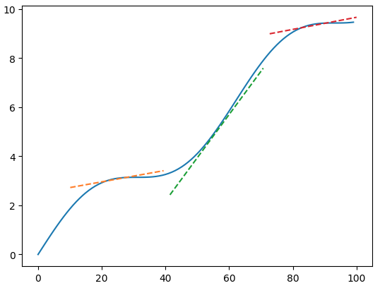
Here, we generated the curve using the equation x + sin(x). You will notice that the resulting curve somewhat resembles stock price fluctuations. This is not surprising, as stock price fluctuations can essentially be decomposed into a DC component and a superposition of many sine waves. The DC component reflects the company's ongoing operational capability, while the sine waves reflect the traces left by short-term speculative funds operating on the asset.

Returning to our main topic. Now, let's remove the plotting functionality and test how long this code takes to execute:

1234567891011121314x = np.linspace(0, 100, 100)
y = np.sin(x/10) + x/10

def moving_lsq(ts, win: int):
    x = np.arange(len(ts))
    S = []
    for i in range(win, len(ts)):
        xi = x[i-win:i]
        yi = ts[i-win:i]
        fitted = Polynomial.fit(xi, yi, deg=1, domain=[])
        S.append(fitted.coef[1])
    return S

%timeit moving_lsq(y, 10)

90 loops took a total of 25ms. Considering that there are over 5,000 stocks in China A-shares, calculating all of them once would take more than 2 minutes.

To accelerate this calculation process, we must rely on vectorization. However, this time, there is no magical API to call; we must roll up our sleeves and start from understanding the underlying mathematical principles to create our own implementation.

Vectorization

Considering a linear regression with m points, for each point, we have:

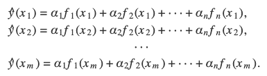
If all points fall on the same line, the following matrix equation holds:

$$ Y = A\beta + b $$

Here, $A$ is $X$, and $\beta$ is the coefficient to be solved:

$$ \beta = {(A^TA)}^{-1}A^TY $$

For formula derivation, see 《Python programming and Numerical Methods - A Guide for Engineers and Scientists》

We can manually verify this formula:

1234567891011x = np.linspace(0, 9, 10)
y = x + np.sin(x/10)

win = 10

A = np.arange(win).reshape((win,1))
pinv = np.dot(np.linalg.inv(np.dot(A.T, A)), A.T)
alpha_1 = np.dot(pinv, y[:, np.newaxis]).item()
alpha_2 = Polynomial.fit(x, y, deg=1, domain=[]).coef[1]

np.isclose(alpha_1, alpha_2, atol=1e-2)

We solved for the slope using two methods, and the results show that under an absolute error constraint of 1e-2, they are identical.

Note that in line 7, we used the variable name pinv. This is because there is a function with the same name in numpy.linalg, which exactly calculates ${(A^TA)}^{-1}A^T$.

However, so far, we have only accomplished what Polynomial.fit does. If we want to calculate the slopes of fitted lines for all sliding windows at once, how should we proceed?

Note that we calculate the slope through a matrix multiplication. In Numpy, matrix multiplication is inherently vectorized. In line 7, pinv is a (1,10) matrix, and $y$ is a (10,) vector. If we can stack the corresponding pinv for each group under the sliding window and stack $y$ into a matrix, we can calculate all slopes at once through matrix multiplication.

Let's start with y. When we slide y = np.arange(5) with a window size of 3, we essentially obtain the following matrix:

$$ \begin{bmatrix}0&1&2\1&2&3\2&3&4\\end{bmatrix} $$

To obtain this matrix, we can use fancy indexing:

12345y[
    [0, 1, 2],
    [1, 2, 3],
    [2, 3, 4]
]

Therefore, to implement the matrix of $y$ under a sliding window, we only need to construct this fancy index matrix. The good news is that the fancy index matrix is very regular:

12345678910111213141516def extract_windows_vectorized(array, win:int):
    start = 0
    max = len(array) - win + 1
    
    sub_windows = (
        start +
        # expand_dims are used to convert a 1D array to 2D array.
        np.expand_dims(np.arange(win), 0) +
        np.expand_dims(np.arange(max), 0).T
    )

    return array[sub_windows]

arr_1d = np.arange(10, 20)

extract_windows_vectorized(arr_1d, 4)

If you find this method difficult to understand, Numpy already provides a function named as_strided that can achieve our functionality in one step and is faster (by a factor of 2) than the above method:

123456789from numpy.lib.stride_tricks import as_strided

y = np.arange(3, 10)
stride = y.strdies[0]

win = 4
shape = (len(y) - win + 1, win)
strides = (stride, stride)
as_strided(y, shape, strides)

The matrix pinv is generated from $x$. If the time series $y$ is 100 periods long, the values of $x$ will range from 0 to 99.

Where $[x0, x1, ..., x_{win-1}]$ corresponds to $[y0, y1, ..., y_{win-1}]$, $[x1, x2, ..., x_{win}]$ corresponds to $[y1, y2, ..., y_{win}]$, and $[x_{-win}, x_{-win+1}, ... x_{-1}]$ corresponds to $[y_{-win}, y_{-win+1}, ..., y_{-1}]$.

Therefore, the coefficient matrix $A$ we need to construct is:

12A = as_strided(np.arange(len(y)), shape, strides)
pinv = np.linalg.pinv(A)

The subsequent regression operations are the same as before:

1alpha = pinv.dot(y).sum(axis = 0)

The complete code is as follows:

12345678910def moving_lsq_vector(ts, win:int):
    stride = ts.strides[0]

    strides = (stride, stride)
    shape = (win,len(ts)-win+1)
    A = as_strided(np.arange(len(ts)), shape= shape, strides=strides)
    pinv = np.linalg.pinv(A)
    y = as_strided(ts, shape=shape, strides = strides)
    
    return pinv.dot(y).sum(axis=0)

This version is 100 times faster than the previous one using Polynomial.fit plus a loop. You may have guessed that this 100x speedup is approximately equal to the number of iterations. This is the cost of looping.

Now, can we use the method here to accelerate other calculations? The answer is obviously yes. If you need to quickly calculate the 5-day moving average for the past 10 days for 5,000 stocks, after obtaining the recent 14 days of stock prices, you form a (5000, 14) matrix $A$. Now, all you need to do is convert this matrix into a 3D matrix and then multiply it by a convolution kernel:

1234567891011121314151617from numpy.typing import NDArray
def batch_move_mean(A: NDArray, win:int)->NDArray:
    """批量计算移动平均线

    Args:
        A: (m*n)的价格矩阵。m为股票支数
        win: 移动平均窗口
    Returns:
        （m * (n-win+1))的矩阵.
    """
    kernel = np.ones(win)/win
    
    s0, s1 = prices.strides
    m, n = prices.shape

    pm = as_strided(prices, shape=(m, n-win + 1, win), strides=(s0, s1, s1))
    return np.dot(pm, kernel.T).squeeze()

We test it with the following code:

123456prices = np.array([
    np.arange(0, 14),
    np.arange(10, 24)
])

batch_move_mean(prices, 5)

The output is:

12array([[ 2.,  3.,  4.,  5.,  6.,  7.,  8.,  9., 10., 11.],
       [12., 13., 14., 15., 16., 17., 18., 19., 20., 21.]])

As expected, but lightning fast.

Aside

Should we use fitted trend lines as a momentum factor? This is a topic worth discussing in depth. The biggest problem with slope factors is not that all time series have obvious trends. Mathematically, if the fitting residuals are large, it indicates that the time series has not yet formed an obvious trend, and thus the slope factor should not be used. Another issue is the old problem of linear regression, where individual outliers have a significant impact on the fit. Should the fitted line minimize the sum of distances from all points to the line, or should it minimize the sum of distances for the majority of points (which is less than the former)?

Conclusion

We discussed how to perform linear regression (line fitting) using Numpy and introduced the latest polynomial API. Then, we introduced how to use matrix operations to achieve vectorization.

The core point is to use the as_strided method to upsize the array, and then perform matrix operations on the up-sized array to achieve vectorization. We also used the same approach to solve the problem of calculating the moving average for 5,000 stocks at once. You also saw a practical example of fancy indexing. This chapter contains many techniques and serves as a summary of previous chapters.