Numpy Quant: Median Clipping, VWAP, Rolling MDD
This Week's Highlights
- Mortgage rates for existing loans adjusted downward starting Oct 25!
- Robotaxi Day ends abruptly; Tesla stock plummets
- Incremental fiscal policy package exceeds expectations, potentially exceeding 5 trillion RMB
- Debt-resolution concepts emerge!
Next Week's Watchlist
- Sunday: September PPI and CPI data released
- Monday (Oct 14): State Council Information Office holds press conference on Q1-Q3 import/export data
This Week's Selection
- Series! Numpy Programming Essentials for Quants (Part 6)
- ICBC released a FAQ on the adjustment of existing mortgage rates, revealing that most existing housing loans can be adjusted to no less than LPR minus 30 basis points (excluding second homes in Beijing, Shanghai, and Shenzhen), with a unified batch adjustment on October 25. Assuming a 1 million RMB loan, 25-year term, and equal principal and interest repayment, the adjustment saves 469 RMB per month, totaling 140,600 RMB in interest savings.
- The "We Robot" event was held, which Musk previously called "historic." However, the curtain rose on a brief 20-minute keynote presentation, with no key technical indicators or parameters disclosed. Tesla subsequently fell 8.78%, while its competitor Lyft surged 9.59%.
- The Ministry of Finance held a press conference on Saturday, unveiling a package of incremental fiscal policies. Analysts conservatively estimate the scale of this package at over 5 trillion RMB, focusing on debt resolution and ensuring basic government operations at the grassroots level.
- Following the Ministry of Finance's announcement, debt-resolution concepts sparked market热议. Securities Times Data Hub梳理ed that approximately 37 companies in AMC, city investment platforms, PPP concepts, and REITs concepts may benefit. Despite the sharp market drop on Friday, most of these companies rose against the trend or outperformed the broader market.
Numpy Quant Application Cases [3]
Vectorization Example: Median-Based Outlier Clipping for Multi-Assets
Outlier clipping is a common step in quantitative analysis preprocessing and is also prevalent in machine learning. Among various outlier clipping methods, median-based clipping (pulling back to the median) is the most adaptable and robust to different data distribution characteristics.
First, let's introduce the concept of Median Absolute Deviation (MAD):
$$MAD = median(|X_i - median(X)|)$$
To treat MAD as an estimator consistent with the standard deviation $\sigma$, i.e., $$\hat{\sigma} = k \cdot MAD$$
Here, $k$ is a proportionality constant. If the distribution is normal, we can calculate: $$ k = \frac{1}{\Phi^{-1}(\frac{3}{4})} \approx 1.4826 $$
Based on this $k$ value, taking 3 times MAD approximates to 5 times the standard deviation.
The code implementation is as follows:
from numpy.typing import ArrayLike
def mad_clip(arr: ArrayLike, k: int = 3):
med = np.median(arr)
mad = np.median(np.abs(arr - med))
return np.clip(arr, med - k * mad, med + k * mad)
np.random.seed(78)
arr = np.append(np.random.randint(1, 4, 20), [15, -10])
mad_clip(arr, 3)This code only performs mad_clip on a single asset. If we need to clip outliers for a specific metric across all A-shares simultaneously, the above method would require looping over 5,000 times, which is obviously slow. In such cases, we can use the following method:
def mad_clip(df: Union[NDArray, pd.DataFrame], k: int = 3, axis=1):
"""使用 MAD 3 倍截断法去极值"""
med = np.median(df, axis=axis).reshape(df.shape[0], -1)
mad = np.median(np.abs(df - med), axis=axis)
magic = 1.4826
offset = k * magic * mad
med = med.flatten()
return np.clip(df.T, med - offset, med + offset).TThis version of mad_clip accepts both numpy ndarray and pandas dataframe as parameters. The output format matches the input format.
We passed the axis parameter in the np.median call. If axis=0, it traverses column-wise, meaning it takes the median across rows (i.e., for each date across assets). If axis=1, it traverses row-wise, meaning it takes the median across columns (i.e., for each asset across dates).
Let's test this with real data:
# 加载测试数据
start = datetime.date(2023, 1, 1)
end = datetime.date(2023, 12, 29)
barss = load_bars(start, end, 7)
closes = barss["close"].unstack("asset").iloc[-5:]
closesThe output data is:
| asset/date | 002095.XSHE | 003042.XSHE | 300099.XSHE | 301060.XSHE | 601689.XSHG | 603255.XSHG | 688669.XSHG |
|---|---|---|---|---|---|---|---|
| 2023-12-25 | 23.400000 | 18.090000 | 6.10 | 13.00 | 73.910004 | 36.799999 | 18.080000 |
| 2023-12-26 | 21.059999 | 17.520000 | 5.94 | 12.83 | 72.879997 | 37.000000 | 18.080000 |
| 2023-12-27 | 20.070000 | 17.590000 | 6.04 | 12.84 | 72.000000 | 36.840000 | 18.049999 |
| 2023-12-28 | 20.010000 | 18.139999 | 6.11 | 13.14 | 72.199997 | 38.150002 | 18.440001 |
| 2023-12-29 | 20.270000 | 18.580000 | 6.19 | 13.29 | 73.500000 | 37.299999 | 18.740000 |
To test the effect, we set $k$ to a smaller value to observe the impact:
mad_clip(closes,k=1)| asset/date | 002095.XSHE | 003042.XSHE | 300099.XSHE | 301060.XSHE | 601689.XSHG | 603255.XSHG | 688669.XSHG |
|---|---|---|---|---|---|---|---|
| 2023-12-25 | 23.400000 | 18.090000 | 10.217396 | 13.00 | 25.962605 | 25.962605 | 18.080000 |
| 2023-12-26 | 21.059999 | 17.520000 | 10.296350 | 12.83 | 25.863649 | 25.863649 | 18.080000 |
| 2023-12-27 | 20.070000 | 17.590000 | 10.325655 | 12.84 | 25.774343 | 25.774343 | 18.049999 |
| 2023-12-28 | 20.010000 | 18.139999 | 10.582220 | 13.14 | 26.297781 | 26.297781 | 18.440001 |
| 2023-12-29 | 20.270000 | 18.580000 | 10.659830 | 13.29 | 26.820169 | 26.820169 | 18.740000 |
We observe that the original value of 73.9 was pulled back to 25.9, and 6.1 was pulled back to 10.2 (taking the first row as an example), and these calculations are performed row by row (i.e., per asset per date).
min_range: What is the minimum value over the past N periods?
This is a very common requirement. For instance, there is a stock market proverb: "Huge volume marks the top, tiny volume marks the bottom." When the market is at a high level, if trading volume hits a multi-period high (huge volume), subsequent volume may struggle to sustain, potentially leading to a decline. When the market is at a low level, if trading volume hits a multi-period low (tiny volume), it indicates extremely low market sentiment, making prices susceptible to manipulation and attracting speculative capital.
This function exists in TongDaXin formulas, and in MaiYan language, the corresponding method might be LOWRANGE. Below is the implementation of the LowRange function in myTT:
def LOWRANGE(S):
# LOWRANGE(LOW)表示当前最低价是近多少周期内最低价的最小值 by jqz1226
rt = np.zeros(len(S))
for i in range(1,len(S)): rt[i] = np.argmin(np.flipud(S[:i]>S[i]))
return rt.astype('int')This appears simple but is actually difficult to implement correctly. If we test the above function, we will find that it may not meet the requirements (or it could be that the author of this article misunderstood the function).
s = [ 1, 2, 2, 1, 3, 0]
LOWRANGE(np.array(s))In the above test, we expected the output to be [1, 1, 1, 3, 1, 6], but LOWRANG would produce the following output:
array([0, 0, 0, 2, 0, 0])Below, we provide a vectorized implementation of this function.
warning
This function may produce incorrect outputs for the first few elements. Since it does not affect factor analysis, it has not been fixed yet.def min_range(s):
"""计算序列s中,元素i是此前多少个周期以来的最小值
此方法在个别数字上有bug
Example:
>>> s = np.array([5, 7, 7, 6, 5, 8, 2])
>>> min_range(s)
array([1, 2, 1, 2, 3, 1, 6])
"""
n = len(s)
# handle nan
filled = np.where(np.isnan(s), -np.inf, s)
diff = filled[:,None] - filled
mask = np.triu(np.ones((n, n), dtype=bool), k=1)
masked = np.ma.array(diff, mask=mask)
rng = np.arange(n)
ret = rng - np.argmax(np.ma.where(masked > 0, rng, -1), axis=1)
ret[0] = 1
if filled[1] <= filled[0]:
ret[1] = 2
return ret
s = np.array([5, 7, 7, 6, 5, 8, 2])
min_range(s)The final output result is:
array([1, 1, 2, 3, 4, 1, 6])At the position of the second 7, the output is inconsistent with expectations, but subsequent calculations are correct. This implementation is quite clever, using a triangular matrix mask array to eliminate loops.
Moving Average Calculation: SMA and Intraday VWAP
Calculating moving averages using Numpy is simple; you can use np.convolve().
def moving_average(ts: ArrayLike, win: int, padding=True)->np.ndarray:
kernel = np.ones(win) / win
arr = np.convolve(ts, kernel, 'valid')
if padding:
return np.insert(arr, 0, [np.nan] * (win - 1))
else:
return arr
moving_average(np.arange(5), 3)The output result is array([nan, nan, 1., 2., 3.])
Moving averages consider only price information. The intraday volume-weighted average price (VWAP), however, incorporates both volume and price information, holding special significance for intraday trading. For example, in a poor market environment, if a stock's price is below the intraday VWAP and has failed to break above it twice, a third failure is generally considered a signal to sell quickly. Conversely, similar logic applies to buying.
The calculation of the VWAP is as follows:
If the current time is $t$, the cumulative average transaction price at that moment is obtained by dividing the total transaction amount from the open until time $t$ by the total volume. Connecting the average transaction prices at all moments forms the intraday VWAP.
This feature seems complex, but since Numpy provides the cumsum function, the actual calculation is very simple:
def intraday_moving_average(bars: DataFrame)->np.ndarray:
acc_vol = bars["volume"].cumsum()
acc_money = barss["amount"].cumsum()
return acc_money / acc_volIn this environment, only daily data is provided, so we use daily data to test instead of minute-level data:
start = datetime.date(2023, 1, 1)
end = datetime.date(2023, 12, 29)
barss = load_bars(start, end, 1)
intraday_moving_average(barss)Calculating Maximum Drawdown
Maximum Drawdown (MDD) refers to the maximum observed loss from a peak to a trough of a portfolio, until a new peak is reached. MDD is a downside risk indicator over a certain time period.
$$ MDD = \frac{Trough Value - Peak Value}{Peak Value} $$
Max drawdown is an important indicator for measuring investment strategy risk. Therefore, it is implemented in the empyrical library. However, as a strategy risk assessment indicator, empyrical does not need to return information such as duration, nor does it implement MDD under a sliding window. Now, let's implement the rolling version.
# https://stackoverflow.com/a/21059308
from numpy.lib.stride_tricks import as_strided
import matplotlib.pyplot as plt
def windowed_view(x, window_size):
"""Creat a 2d windowed view of a 1d array.
`x` must be a 1d numpy array.
`numpy.lib.stride_tricks.as_strided` is used to create the view.
The data is not copied.
Example:
>>> x = np.array([1, 2, 3, 4, 5, 6])
>>> windowed_view(x, 3)
array([[1, 2, 3],
[2, 3, 4],
[3, 4, 5],
[4, 5, 6]])
"""
y = as_strided(x, shape=(x.size - window_size + 1, window_size),
strides=(x.strides[0], x.strides[0]))
return ydef rolling_max_dd(x, window_size, min_periods=1):
"""Compute the rolling maximum drawdown of `x`.
`x` must be a 1d numpy array.
`min_periods` should satisfy `1 <= min_periods <= window_size`.
Returns an 1d array with length `len(x) - min_periods + 1`.
"""
if min_periods < window_size:
pad = np.empty(window_size - min_periods)
pad.fill(x[0])
x = np.concatenate((pad, x))
y = windowed_view(x, window_size)
running_max_y = np.maximum.accumulate(y, axis=1)
dd = y - running_max_y
return dd.min(axis=1)
np.random.seed(0)
n = 100
s = np.random.randn(n).cumsum()
win = 20
mdd = rolling_max_dd(s, win, min_periods=1)
plt.plot(s, 'b')
plt.plot(mdd, 'g.')
plt.show()Testing shows that when the time series $s$ has a length of 1000, the calculation time for rolling_max_dd is 100$\mu$S.
The comparison chart of MDD generated under a sliding window versus the original sequence is as follows:
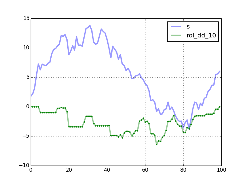
This method also simply encapsulates a function to convert a 1D array into a sliding window view, which can be used elsewhere.
Finding Adaptive Parameters
Many trading strategies based on technical indicators specify fixed thresholds. For example, some people short when RSI is above 80 and go long when RSI is below 20. Even when applied to indices and industry sectors, such indicators are still not precise enough because, in an upward channel, RSI peaks will be higher than RSI peaks in a downward channel; in a downward channel, RSI bottoms will be much lower than RSI bottoms in an upward channel.
Furthermore, different assets have different RSI value ranges. Not just RSI, many technical indicators require adaptive parameters based on the current market environment and the specific asset.
One solution is to use a Bollinger Bands-like approach, using the upper and lower bounds of the standard deviation of the indicator's mean. However, this approach implicitly assumes that the data distribution of the indicator's mean follows a normal distribution.
We can relax this condition and instead use percentiles, i.e., Numpy's percentile, to determine parameter thresholds.
%precision 2
from IPython.core.interactiveshell import InteractiveShell
InteractiveShell.ast_node_interactivity = "all"
np.random.seed(78)
s = np.random.randn(100)
hbound = np.percentile(s, 95)
lbound = np.percentile(s, 5)
s[s> hbound]
s[s< lbound]By using percentile to find data exceeding the upper and lower bounds, the output is as follows:
array([2.09, 2.27, 2.21, 2.12, 2.19])
array([-1.68, -2.4 , -1.97, -1.7 , -1.46])Once the indicator exceeds the 95% percentile (hbound), we short; once the indicator falls below the 5% percentile (lbound), we go long.
Here, we can also use the median-based outlier clipping method. Once the indicator exceeds 3 times the MAD value of the median, a trading signal is issued.
"Factor Investing and Machine Learning Strategies" Course is Now Open!

Clear Goals, Strong Sense of Achievement

Why You Should Take QuanTide's Course?