
Why Peak Detection Fails in Live Trading: A Look at SciPy
SciPy provides signal-processing utilities, such as argrelextrema, that can identify market tops and bottoms. Judging by its name, this function locates the coordinates of relative extrema. Let’s examine how it works:
def bs_signals(bars):
from scipy.signal import argrelextrema
ma = moving_average(bars["close"], 5)
peak_indexes = argrelextrema(ma, np.greater)
peaks = peak_indexes[0]
# Find valleys(min).
valley_indexes = argrelextrema(ma, np.less)
valleys = valley_indexes[0]
assert abs(len(peaks) - len(valleys)) <= 1
bars = bars[4:]
# Plot main graph.
(fig, ax) = plt.subplots()
ax.plot(np.arange(len(bars)), bars["close"], color='c')
ax.plot(np.arange(len(bars)), ma, color='b')
# Plot peaks.
peak_x = peaks
peak_y = bars['close'][peak_x]
ax.plot(peak_x, peak_y, 'gv', label="Peaks")
# Plot valleys.
valley_x = valleys
valley_y = bars['close'][valley_x]
ax.plot(valley_x, valley_y, 'r^', label="Valleys")
trades = []
gains = 1
order = None
vertex = sorted([*peaks, *valleys])
for x in vertex:
buy = x in valleys
sell = x in peaks
if buy and order is None:
order = {
"buy": bars["close"][x],
"buy_at": bars["frame"][x]
}
elif sell and order:
buy = order["buy"]
sell = bars["close"][x]
gain = sell / buy
order.update({
"sell": sell,
"sell_at": bars["frame"][x],
"gain": gain
})
gains *= gain
trades.append(order)
order = None
return gains - 1, tradesThe code above uses argrelextrema to find peaks and valleys in a moving average. We use a moving average because it smooths out noise. Here, moving_average is defined as:
import numpy as np
def moving_average(ts, win):
return np.convolve(ts, np.ones(win) / win, mode="valid")It employs convolution to compute the simple moving average. While NumPy’s convolution is fast, you can achieve significantly higher performance using move_mean from bottleneck—up to 6,000 times faster in some benchmarks (per official documentation, though comparisons with np.convolve may vary).
By passing different comparison functions (e.g., np.less and np.greater) to argrelextrema, we can separately identify local maxima and minima, labeled as peaks and valleys.
We then plot the moving average, closing prices, and detected extrema on the same chart. Finally, assuming we buy at the lows and sell at the highs, we can calculate the strategy’s returns.
The figure below shows the signal detection results for Dongfang Electric over a 60-trading-day window, ending on November 2, 2021:
As shown, even with default parameters, argrelextrema identifies tops and bottoms reasonably well. Our final return was 35%, while the stock itself remained flat over the same period.
Impressive, but too good to be true.
So, where is the flaw?
The issue lies in how argrelextrema operates. It can only detect a peak after the price has already started to decline. This makes it a look-ahead function. It implies that the signal for today might only be identifiable tomorrow. But we cannot travel back in time to execute trades yesterday.
To further validate this, let’s compare two snapshots around September 3, 2021:
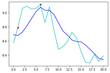 The first image shows the chart up to September 3. Based on subsequent price action,
 argrelextrema should have flagged a bottom on this day. It did not.
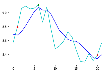 The second image is dated September 6. This time, it flagged a bottom, but the label appears one day earlier than the actual price low.
Since the moving average is calculated using closing prices, we can only identify September 3 as a low point after the market closes on September 6. If we were to buy at the September 6 closing price (or, in live trading, the next day’s open), what would happen?
By shifting both entry and exit prices by one day, the resulting return drops to -13%. If we had simply bought at the open on the start date and sold at the close on the end date, we would have gained 8.4%. After applying sophisticated mathematical methods, we successfully lost 21%. This was using a 5-day moving average. Using 10-day or 3-day averages yields similar losses.
Ideally, it works perfectly. In reality, it’s harsh.
However...
Experienced traders often notice that around position 5, the price stalls for several days, and the moving average flattens. A common market adage states: “If it doesn’t hit a new high in three days, sell” (particularly for strong momentum stocks). This is because if the price fails to make new highs, the moving average flattens as seen near position 5. From there, the price may either break out to start a second wave or decline.
Thus, our strategy could be adjusted: use the algorithm to detect when the moving average flattens and issue a warning (e.g., partially reduce position), then wait for a confirmed signal before clearing the entire position (or, conversely, buying).
Assume we can detect the flattening signal one day before argrelextrema flags the peak. If we are at a high, we sell half the position. Once argrelextrema confirms the signal, we sell the remainder. This modifies the entry and exit logic as follows:
if buy and order is None:
order = {
"buy": close[x] * 0.5 + close[x+1] * 0.5,
"buy_at": bars["frame"][x+1]
}
elif sell and order:
buy = order["buy"]
sell = close[x+1] * 0.5 + close[x] * 0.5,
gain = sell / buy
order.update({
"sell": sell,
"sell_at": bars["frame"][x+1],
"gain": gain
})With this adjustment, our return is 5%. While lower than a simple buy-and-hold, this is income earned through skill rather than luck, making it reproducible.
The question now becomes: how do we detect a flattening moving average? This is not trivial. However, let’s first clarify the actual utility of the peak and valley detection method discussed here.
As analyzed, peak and valley detection is ex-post: the algorithm can only detect extrema after they have formed. While this may not offer direct trading guidance, we can use these signals to label data for machine learning.
The figure below shows the results of labeling peaks and valleys on the Shanghai Composite Index over a specific period using the above method:
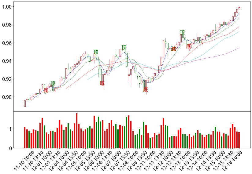
We first smooth volatility using a moving average, then detect peaks and valleys via argrelextrema. Finally, we make minor adjustments to align the labeled points with the actual stock price rather than the moving average. Using 30-minute data for the Shanghai Index over the past six years, we identified 734 peaks and 738 valleys, creating a labeled dataset.
With this labeled data, we can train and validate our machine learning models. Surprisingly, the dataset is not large. This suggests that in China A-shares, once a trend forms, it often persists for some time. This also highlights why quantitative models remain effective in this market.