Portfolio Theory & Practice (2): Monte Carlo Optimization

Monte Carlo simulation involves randomly generating a large number of asset allocation schemes, calculating the resulting volatility and Sharpe ratio for each, and then reverse-engineering the allocation scheme based on the optimal Sharpe ratio.

The primary operations were introduced in the previous section; this step primarily involves repeating these operations. We present the code first, followed by an explanation:

12345678910111213141516171819202122num_ports = 5000

w = np.zeros((num_ports, len(stocks)))
vol_arr = np.zeros(num_ports)
sharpe_arr = np.zeros(num_ports)
port_return_arr = np.zeros((num_ports, len(returns)))
cov_arr = np.zeros(num_ports)

for i in range(num_ports):
    weights = np.array(np.random.random(len(stocks)))
    weights = weights/np.sum(weights)  
                    
    w[i,:] = weights
  
    weighted_returns = weights * returns
    port_return_i = weighted_returns.sum(axis=1)
    port_return_arr[i,:] = port_return_i

    cov = np.cov(port_return_i)
    cov_arr[i] = cov
    vol_arr[i] = np.sqrt(np.dot(weights.T, np.dot(cov, weights)))
    sharpe_arr[i] = sharpe_ratio(port_return_i)

We define four main arrays:

1. all_weights: A weight matrix. We plan to repeat the sampling 5,000 times. Since the portfolio consists of 4 assets, this is a 5000 * 4 matrix. Each row corresponds to one asset allocation scheme.
2. sharpe_arr: An array of size 5000, recording the calculated Sharpe ratio for each iteration.
3. vol_arr: An array of size 5000, recording the calculated volatility for each iteration.
4. port_return_arr: In the example, this is a 5000 * 241 matrix, where each row records the portfolio's daily returns over the past year.

Once the code execution is complete, we obtain 5,000 sets of Sharpe values. According to the definition of the Sharpe ratio, the set with the maximum Sharpe value represents the asset allocation with the highest return for the lowest risk.

Determining the Optimal Portfolio

We use np.argmax to locate the position of the maximum Sharpe ratio, which identifies the optimal portfolio:

12345# 检查最高的 SHARPE
pos = np.argmax(sharpe_arr)
print(pos, sharpe_arr[pos])
print("stocks", stocks)
print("Portfolio Allocation:", w[pos])

This yields an asset allocation scheme similar to the following:

	Asset 1	Asset 2	Asset 3	Asset 4
Weight	35.3%	0.3%	0.8%	64%

We plot the results of the above experiment to see if they align with the Efficient Frontier theory:

1234567import matplotlib.pyplot as plt

annual_return = np.prod((1 + port_return_arr), axis=1) - 1
plt.scatter(vol_arr, annual_return, c=sharpe_arr, cmap='RdYlBu')
plt.colorbar(label='Sharpe Ratio')

plt.scatter(vol_arr[pos], annual_return[pos], c='red',s=80)

We use volatility as the x-axis and annualized return as the y-axis. For each x, there are multiple annualized return data points, both positive and negative. Clearly, for the same x, the combinations on the efficient frontier are those with the maximum return or maximum loss.

According to Modern Portfolio Theory (MPT), only combinations above the y-axis and on the efficient frontier are worth considering. We then select the corresponding combination on this line based on our risk tolerance.

We mark the scheme with the highest Sharpe ratio with a red dot.

From the trend chart, the asset portfolio we derived is indeed optimal. However, if we compare it with the chart at the beginning of the article, what conclusion do we draw?

1. The hand is weak. If you are willing to take significant risk, this hand still cannot provide the desired returns. The volatility is not high enough.
2. The portfolio does not form an intuitive efficient frontier. This is mainly because the portfolio's overall return is constrained by the returns of the assets within it: $min(return_{assets}) \le return_{portfolio} \le max(return_{assets})$. Therefore, not all returns are achievable.

Thus, we reach the conclusion: You need to re-select your assets.

Additionally, if you are eager to use MPT for investing right now... you still have more to learn.

History certainly repeats itself; all history is contemporary history. However, there is still much to discuss.

First, how many assets should we include in this portfolio? Our example used only 4. Would it be better to conduct index-enhanced strategies on the CSI 300 or CSI 1000?

Second, the two charts above are for the same asset portfolio but under different time periods, showing significant differences in returns and risks. If we optimize the portfolio at different time points, the resulting positions will obviously differ. Therefore, we pose the question: How often should we calculate and execute rebalancing? Is there a scenario where each rebalancing uses the past optimal solution, which quickly becomes suboptimal or even the worst solution? In other words, what is the momentum cycle of this portfolio?

Clearly, any valuable scheme cannot be covered in a short article. We will continue to explore this issue in subsequent articles.

For now, let us set these questions aside and look at a technical issue:

Executing the above loop 5,000 times took approximately 5.2 seconds.

This is for a case with only 4 assets. Obviously, as the number of assets increases, the space for brute-force search also expands. Is this method still feasible when the number of assets increases to 50 or 100?

Before discussing feasibility, we can attempt some speed optimizations.

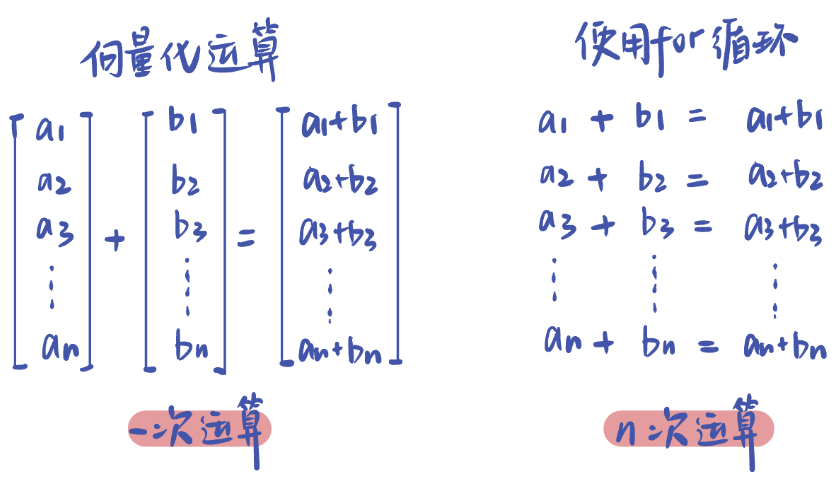
We can use the following algorithm to move some calculations out of the loop:

123456789101112131415161718192021222324252627282930313233343536from empyrical import sharpe_ratio
import time
start = time.time()
num_ports = 5000
all_weights = np.random.rand(num_ports, len(stocks))

shape = (len(all_weights), -1)
all_weights = all_weights/all_weights.sum(axis=1).reshape(shape)

# got 241 daily summed returns over 5000 iters
all_port_returns = np.dot(all_weights,returns.T)

all_cov = np.cov(all_port_returns).diagonal()

# 计算波动率
all_vol = []
all_sharpe = []

annual_return = np.prod((1 + all_port_returns), axis=1) - 1

for i in range(num_ports):
    all_vol.append(np.sqrt(np.dot(all_weights[i].T, np.dot(all_cov[i], all_weights[i]))))
    all_sharpe.append(sharpe_ratio(all_port_returns[i]))

end = time.time()
print("计算用时", end-start)

# 绘图
all_vol = np.array(all_vol)
pos = np.argsort(all_vol)

plt.scatter(all_vol, annual_return, c=all_sharpe, cmap='RdYlBu')
plt.colorbar(label='Sharpe Ratio')

max_sharpe_pos = np.argmax(all_sharpe)
plt.scatter(all_vol[max_sharpe_pos], annual_return[max_sharpe_pos], c='red',s=80)

However, when calculating volatility and Sharpe ratio row by row, I had to compromise and use loops. In this case (with only 4 assets in the portfolio), the current execution time is 0.65 seconds. This represents an approximately 8-fold speed improvement (from an initial ~5.2s).

The author of PyPortfolioOpt used a similar method in an example:

12345n_samples = 10000
w = np.random.dirichlet(np.ones(ef.n_assets), n_samples)
rets = w.dot(ef.expected_returns)
stds = np.sqrt(np.diag(w @ ef.cov_matrix @ w.T))
sharpes = rets / stds

The calculation speed is very fast (less than 0.1 seconds), but it requires replacing ef.cov_matrix. Interested readers can study its source code.

For a portfolio with only 4 assets, this speed (under 1 second) is obviously satisfactory. However, as mentioned in the previous article, as the number of assets increases, the search space for Monte Carlo simulation also expands. How much will it increase, and is it still feasible?

Let us first look at the case with only two assets. Assume the interval for asset weights is 1%, meaning an asset is allocated either 1% or 2%, but not non-integer weights like 1.05%. In this way, we can calculate that if we want to simulate all these weight distributions, the search space will be:

A: 1-100 ~ 101 options B: 1 option

Once the weight for A is determined, under the constraint that the sum of weights equals 1, B has only one choice. Therefore, the total number of searches is 101.

As the number of assets increases, to simulate as many cases as possible, we must increase the number of simulations, causing the total runtime to rise rapidly. Moreover, as the number of assets increases, the number of searches required increases exponentially, not linearly with the number of assets.

Therefore, the number of searches is a combinatorial problem. Assuming there are four assets, it is not simply 4×100 that can simulate all combinations, but rather: $C_{99}^3$ allocation schemes.

For any $n$ assets, if the weight interval for each asset is calculated at 1%, the search space will be:

$C_{101-(n-1)}^{n-1}$ searches. If we have 50 assets, we need to search at least 1.998e+21 times!

You can use `math.comb` to calculate the number of combinations.

Thus, using the Monte Carlo method carries the possibility of failing to exhaust all sample spaces. We must adopt mathematical methods to optimize this solving process.