
Is a Higher Sharpe Ratio Always Better? Three Blind Spots
In quant circles and fund due diligence, the Sharpe ratio enjoys something close to a free pass. Most people open a backtest report and go straight for that one number: above 1.5 is a pass, above 2.0 is excellent, and anything north of 3.0 makes them want to sell the house and pile in.
But if you were handed the two strategies below (assume a risk-free rate of $R_f = 2%$), where would you actually put real money?
| Strategy | Annualized return | Annualized volatility | Sharpe ratio | Max drawdown |
|---|---|---|---|---|
| A | 8% | 4% | 1.5 | -8% |
| B | 20% | 15% | 1.2 | -35% |
Rank purely by Sharpe and A wins hands down. But if your goal is to quintuple your capital over ten years and you can stomach a 30%-plus drawdown along the way, A's 8% annualized return will feel like watching paint dry. Conversely, if you're managing money you'll need in a year to buy a house or meet a redemption, and B's 35% drawdown lands halfway through, that paper "high return" is a disaster for you.
This is why we can't simply say "the higher the Sharpe ratio, the better the strategy." It answers one question precisely — how much excess return each unit of total volatility buys — while staying silent on three questions that decide everything: where the return comes from, how much you can lose in the worst case, and whether you can actually hold on to the position.
/01 Volatility isn't risk, and a long holding period won't dissolve drawdowns
Back to the definition:
$$ Sharpe=\frac{E(R_p)-R_f}{\sigma_p} $$
where $E(R_p)$ is the strategy's average return, $R_f$ is the risk-free rate, and $\sigma_p$ is the standard deviation of returns. It is essentially a value-for-money metric: total volatility in the denominator, excess return in the numerator. It works well as a first-pass screen between strategies that share the same investment horizon, transaction costs, leverage, and sample period — but it must never be treated as a comprehensive score.
Many people see strategy B's 20% annualized return against a Sharpe of only 1.2 and think: volatility is temporary, so if I just extend my holding period, can't I ignore the low Sharpe and the high volatility and collect a steady 20%?
Unfortunately, holding longer doesn't flatten risk automatically; it can expose it more completely.
First, uncertainty about terminal wealth compounds over time. Lengthening the holding period does make the standard deviation of the annualized average return converge at a rate of $1/\sqrt{T}$, but what investors actually care about is how much money is in the account at the end. If period returns are roughly independent, the standard deviation of cumulative return (or log terminal wealth) grows with the square root of time:
$$ \sigma_T \approx \sigma_1\sqrt{T} $$
The longer you hold, the wider the fan of possible terminal wealth. Risk never vanishes into thin air.
Second, the Sharpe ratio conceals the path risk of the equity curve. Two strategies can share an identical annualized return and Sharpe ratio while one spreads small losses evenly across every month and the other grinds through ten straight months of one-way decline in a single year. That's why max drawdown can never be replaced by the Sharpe ratio — it answers "from the historical peak to the subsequent trough, what was the deepest percentage loss the account ever suffered."
"Just hold long term" looks easy on a backtest chart because the code assumes an investor with no emotions and no cash-flow pressure. In the real world, a drawdown period lasting two or three years without recovering principal is enough to make most people capitulate before dawn — from psychological collapse, a family emergency, or a margin call. A strategy that theoretically returns 20% a year, but that you liquidate in tears at a 35% drawdown, leaves you with nothing but a realized loss.
So for strategies with inherently deep drawdown cycles — trend following, CTA, and the like — practitioners routinely bring in the Calmar ratio, which divides annualized return by the absolute value of max drawdown:
$$ Calmar=\frac{Annual\ Return}{|Max\ Drawdown|} $$
Judging a strategy by "how much annualized return per unit of extreme drawdown" usually maps far better onto what ordinary investors actually feel.
/02 It counts a surge as risk while ignoring black swans
Even taken purely at the statistical level, the $\sigma_p$ in the denominator hides two enormous blind spots.
The first is that it treats a surge and a crash as equally risky.
In the standard deviation formula, a month that suddenly earns $+15%$ and another that drops $-15%$ contribute exactly the same amount to the deviation from the mean. In other words, if a strategy climbs steadily and occasionally delivers an upward spike, its volatility $\sigma_p$ gets pushed up significantly, dragging its Sharpe ratio down.
Yet no investor on earth complains that their account "went up too fast." What we truly fear is capital loss and forced liquidation from the downside. To fix this distortion, financial engineering introduced the Sortino ratio, which uses only the downside volatility below a target return ($R_T$, usually $R_f$ or $0$) as the denominator:
$$ Sortino=\frac{E(R_p)-R_T}{\sigma_{\text{downside}}} $$
By stripping out the "penalty" on upside volatility, Sortino measures how much excess return each unit of downside risk buys — clearly a better fit for the real preference: "I don't mind bouncing upward, but I can't accept deep declines."
The second, more lethal blind spot is that the Sharpe ratio is nearly blind to tail risk — the "small gains most of the time, catastrophic loss in extremis" profile.
Picture a strategy that reliably earns $1%$ every month for 99 straight months. Then, in month 100, a liquidity crisis hits and it drops $30%$ in a single month. If a backtest report happens to cover only the first 99 months, you'll see a textbook 45-degree equity curve — volatility near zero, max drawdown negligible, Sharpe ratio off the charts. Even if you include the $-30%$ crash in month 100, the full-sample annualized Sharpe still comes out near $0.8$ — yet the account has already taken a hit severe enough to breach a liquidation line.
This is no paper exercise; it is a script that financial history keeps replaying. Long-Term Capital Management, which blew up in 1998, and XIV, the short-volatility product wiped out overnight in the February 2018 "Volmageddon," both wore towering Sharpe ratios that Wall Street envied for years before their collapse.
Such strategies are everywhere: selling out-of-the-money options, shorting volatility, harvesting high-yield credit spreads, or providing liquidity in asymmetric fashion. People like to describe them as "picking up pennies in front of a steamroller." Their return distribution carries strongly negative skewness and fat tails: collecting a small insurance premium steadily on 99% of days, then giving back years of accumulated principal and profit in one extreme 1% event.
The standard Sharpe ratio uses only the first moment (mean) and second moment (variance) of the return distribution; it simply cannot detect the tail bomb living in the higher moments. If a strategy's dazzling Sharpe exists only because "the sample period happened not to contain that black swan yet," handing it your net worth is carrying firewood to put out a fire.
/03 Leverage can't lift Sharpe, but parameters can fake one
Two myths come up constantly in practice: can you "juice" the Sharpe ratio with leverage or a change in capital size? And how much water is there in the 2.0-plus Sharpe ratios that backtests churn out?
Start with leverage. In the cleanest textbook world — unlimited borrowing at the risk-free rate $R_f$, no fees, no slippage, no margin calls — applying $\lambda$ times leverage gives a portfolio return of $R_{\text{levered}} = R_f + \lambda(R_p - R_f)$. The excess return in the numerator and the volatility in the denominator both scale by exactly $\lambda$:
$$ Sharpe(\lambda)= \frac{\lambda\big(E(R_p)-R_f\big)}{\lambda\sigma_p}
\frac{E(R_p)-R_f}{\sigma_p} $$
The $\lambda$ cancels — in a frictionless ideal model, adding or removing leverage doesn't change the Sharpe ratio at all.
In the real trading world, leverage doesn't just fail to lift Sharpe; it is usually a Sharpe shredder. First, your true financing cost (margin interest, OTC swaps, index-futures basis) is almost always above the risk-free rate $R_f$, and doubled positions and turnover invite heavier impact and slippage — both of which eat directly into the numerator. More fatally, there is forced deleveraging (margin call): when volatility drives the equity curve down, risk limits and margin calls force you to sell at the most panic-stricken, floor-level prices. Once the position is physically wiped out at the bottom, it no longer matters that the market rocketed to new highs three days later. By the same logic, capital size doesn't appear in the Sharpe formula, but once the money hits the strategy's capacity ceiling, market-impact costs degrade the entire return series and drag the live Sharpe ratio down.
Now the second question: is a backtested Sharpe ratio statistically reliable at all?
Many people forget that a backtested Sharpe ratio is not objective truth — it is a sample statistic with sampling error. This hides the most insidious trap in quant research: multiple testing bias.
Even if you run backtests on completely randomly generated fake price series, as long as you sweep 1,000 sets of moving-average or factor parameters on your machine, probability alone will hand you a "holy grail" curve with an in-sample Sharpe above $2.0$. If you show only the luckiest survivor out of those hundreds or thousands of trials, that high Sharpe is essentially overfitting to historical noise. (This is precisely why Marcos López de Prado proposed the Deflated Sharpe Ratio, which discounts for the number of trials.)
There's also the everyday practice of annualizing a daily Sharpe by multiplying by $\sqrt{252}$, which strictly relies on daily returns being independent and identically distributed. If the strategy holds illiquid assets, or daily returns are positively autocorrelated (smoothing effects), a naive $\sqrt{252}$ scaling will substantially overstate the true annualized Sharpe. A high Sharpe quoted in isolation — with no regard for sample length, bull/bear cycle coverage, realistic two-way slippage, and out-of-sample tracking — tends to collapse at the first contact with live trading.
/04 A high-Sharpe soloist is worth less than a low-correlation tile
Since Sharpe, return, and drawdown each have blind spots, how do professional institutions actually choose when these metrics disagree?
In real portfolio management, the decision is never about picking the top name on a one-dimensional leaderboard — it goes through a three-stage funnel.
Stage one is a hard veto. Start with max drawdown, drawdown recovery time, and tail stress tests. If a strategy's historical max drawdown breaches the red line set by the nature of your capital, it is vetoed outright — even at a Sharpe of 2.5 and 40% annualized return. Returns you can't hold through are meaningless to the account.
Stage two is multi-metric alignment. Among all the candidates you can actually hold, line up the Sharpe ratio (efficiency of total volatility), Sortino (efficiency of downside volatility), Calmar (efficiency of extreme drawdown), and the information ratio (active excess efficiency versus the benchmark) and cross-check them. That tells you whether the efficiency comes from durable profit or from tail risk that simply hasn't detonated yet.
Stage three is the great divide between retail and institutions: look at marginal contribution to the portfolio, not at single-strategy rankings.
A stand-alone Sharpe ratio means little on its own. Suppose you already run a CSI 300 long-only equity strategy with a Sharpe of $1.5$, and two new candidates appear: another equity strategy, also with a Sharpe of $1.5$, that rises and falls in lockstep with your existing book; and a commodity CTA or bond strategy with a Sharpe of only $0.8$ that is nearly uncorrelated with equities.
Add the $1.5$-Sharpe same-direction strategy and your portfolio risk isn't diversified at all — overall Sharpe barely moves. Add the $0.8$-Sharpe low-correlation strategy and its peaks and troughs offset those of your existing curve; the combined portfolio's Sharpe may jump above $1.8$.
That's why top portfolio managers never ask "which single Alpha has the highest Sharpe?" They ask: "does this strategy complement what I already hold?" On the portfolio chessboard, low correlation, crisis-time negative correlation, and capital capacity are worth far more than a standalone Sharpe number.
/05 Beyond single-metric worship: building a complete evaluation toolkit
In Lesson 21 of 《量化二十四课》 (Quantitative Investing in 24 Lessons), "Strategy Backtest Evaluation," I devote an entire section to tying this evaluation system together. The reason not to treat the Sharpe ratio as the only answer is that any single metric is just one hand groping at the elephant.
In the course's hands-on code, strategy evaluation has to start with aligning the most basic daily NAV and return conventions — mix simple returns, log returns, cumulative returns, and annualization conventions and every ratio computed downstream is distorted. On that foundation, we put seven yardsticks into one toolbox and let them work together:
- Sharpe Ratio: excess return efficiency per unit of total volatility;
- Sortino Ratio: strips out upside volatility and watches only downside risk;
- Maximum Drawdown: the depth of the worst historical peak-to-trough decline;
- Calmar Ratio: the exchange rate between annualized return and max drawdown;
- Omega Ratio: sets a target return threshold and folds the higher moments of the whole return distribution (skewness, kurtosis) into a probability-weighted ratio of gains to losses;
- Information Ratio: strips out benchmark return and assesses the consistency of active management specifically;
- Alpha / Beta: decomposes whether the money came from market beta exposure or genuine active alpha.
The course also cites a Monte Carlo experiment covering 40 million random return series, answering a brutally practical question: even if you buy a strategy with a genuinely high Sharpe ratio, how much can you still lose along the way?
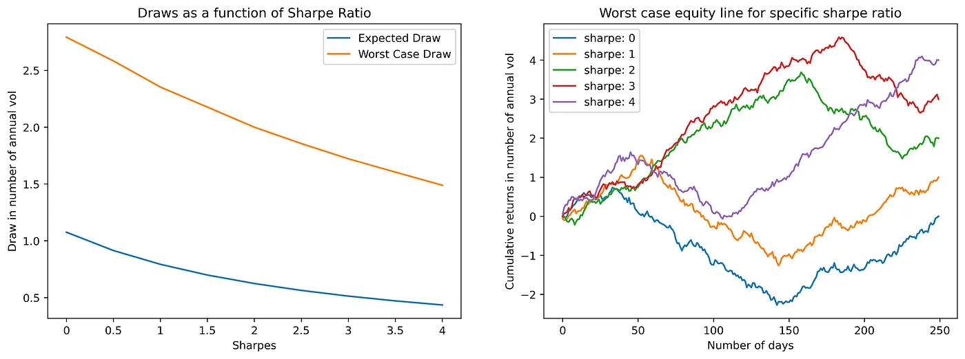
The left panel shows "expected max drawdown" and "worst-case max drawdown" (measured in multiples of annualized volatility) across Sharpe levels; the right panel shows the actual path of the unluckiest equity curve at each Sharpe level.
To make the numbers intuitive, let's plug in a typical equity strategy with 20% annualized volatility (also the most common volatility level for A-share equity funds and the CSI 300 index) and convert the experiment's statistics into real-account max drawdown percentages anyone can read at a glance:
| Sharpe ratio | 0 | 0.5 | 1.0 | 1.5 | 2.0 | 2.5 | 3.0 | 3.5 | 4.0 |
|---|---|---|---|---|---|---|---|---|---|
| Expected max drawdown | -21.6% | -18.2% | -15.8% | -14.0% | -12.4% | -11.2% | -10.2% | -9.4% | -8.8% |
| Worst-case max drawdown | -55.8% | -51.6% | -47.0% | -43.6% | -40.0% | -37.2% | -34.4% | -32.0% | -29.8% |
Faced with these real drawdown percentages, anyone harboring unrealistic fantasies about "high Sharpe" snaps awake:
- A genuinely excellent strategy with a Sharpe of 1.0 (at 20% volatility) still averages a 15.8% drawdown in a normal year; on an unlucky path, its max drawdown within a year can reach -47.0% — nearly half the account.
- Even if you scour the market and buy a top-tier strategy with a true Sharpe of 2.0, you'll still endure an average drawdown of 12.4% — and under an extremely unlucky random path, it can still carve out a -40.0% hole.
- Even at an almost mythical Sharpe of 4.0, you'd still average 8.8% drawdowns, and on a bad run you could still lose close to 30%.
The experiment draws the Sharpe ratio's boundary in sharp relief: Sharpe describes only "risk-exchange efficiency on average." It can never guarantee that the specific historical path you happen to be walking won't suddenly open a 40% hole beneath you.
Back to strategy A (8% annualized, Sharpe 1.5, -8% drawdown) and strategy B (20% annualized, Sharpe 1.2, -35% drawdown) from the opening: you should now be able to give a mature answer. Don't blindly pick A because its Sharpe is higher, and don't impulsively pick B because its return is higher. First, match max drawdown against your capital's time horizon; then dissect both return distributions for the "pennies in front of a steamroller" tail risk; finally, ask which tile makes your existing portfolio more robust.
A high Sharpe ratio only proves that, over that particular slice of history, the strategy was efficient at converting volatility into return. A strategy truly worth entrusting your net worth to is always one whose logic is explainable, whose extreme drawdowns are survivable, whose edge doesn't fade out of sample — and which happens to fit your capital's temperament.
