Here, we introduce a specialized and important library for asset portfolio optimization. Note that we have already discussed the scipy.optimize library. Other similar libraries include cvxopt and cvxpy. However, these are lower-level libraries primarily designed to provide various convex optimization algorithms, not exclusively for the investment domain.

PyPortfolioOpt, on the other hand, is a library dedicated specifically to portfolio optimization. It was originally developed by Robert Martin, a trader, Python enthusiast, and astrophysicist. The library has garnered nearly 4k stars on GitHub.

PyPortfolioOpt provides the following features:

1. Multiple Expected Return Models. For instance, in our previous methods, we used a simple return calculation method, which we can call historical average returns. In earlier parts of this series, we introduced CAPM, which is another form of return. The PyPortfolioOpt library supports not only historical average returns and exponentially weighted historical returns but also CAPM returns. Combining CAPM with Modern Portfolio Theory (MPT) can yield interesting results; you can try this with a small position in your own investments.

2. Risk Models. Previously, we mainly discussed covariance models. PyPortfolioOpt also supports semicovariance (a risk measure focusing on downside changes, aligning with our second requirement), exponential covariance (assigning more weight to recent data), and covariance shrinkage techniques.

3. Objective Functions. PyPortfolioOpt offers Maximum Sharpe Ratio, Minimum Volatility (covered in previous examples), and Maximum Quadratic Utility.

4. Short Selling. It allows holding short positions.

Combining these variations expands the application of MPT in many ways. Perhaps one of these methods will suit the current market. Beyond these optimization methods, there are other common features we need:

1. Visualization. Clearly, we need to plot the covariance matrix, the efficient frontier, and the weight matrix (which is appropriate for pie charts since weights sum to 1).
2. Data Preprocessing and Postprocessing.

After understanding the basic features of PyPortfolioOpt, let’s look at how to use it.

The current version is 1.5.4. Although its basic architecture is stable, maintenance is active, and it supports Python versions from 3.8 to 3.12. It uses Poetry for dependency management.

To install PyPortfolioOpt, use the following command:

1pip install PyPortfolioOpt

It also provides a Docker container (very considerate!) for us to practice with some of its examples.

Next, we will demonstrate the usage of PyPortfolioOpt through an example. In this example, we will show:

1. How to preprocess data into the input format required by PyPortfolioOpt.
2. How to calculate the covariance matrix and visualize it.
3. How to optimize a long-short portfolio to minimize variance.
4. How to maximize the Sharpe ratio.

Data Preprocessing

We use zillionare-omicron to fetch initial data and process it into the input format required by PyPortfolioOpt.

```python from coursea import *

await init()

上证50指数

SH50_CODE_LIST = ["688599.XSHG","688111.XSHG","603986.XSHG","603799.XSHG","603501.XSHG","603288.XSHG", "603260.XSHG","603259.XSHG","601919.XSHG","601899.XSHG","601888.XSHG","601857.XSHG", "601728.XSHG","601669.XSHG","601668.XSHG","601633.XSHG","601628.XSHG","601398.XSHG", "601390.XSHG","601318.XSHG","601288.XSHG","601225.XSHG","601166.XSHG","601088.XSHG", "601066.XSHG","601012.XSHG","600905.XSHG","600900.XSHG","600893.XSHG","600887.XSHG", "600809.XSHG","600745.XSHG","600690.XSHG","600519.XSHG","600438.XSHG","600436.XSHG", "600406.XSHG","600309.XSHG","600276.XSHG","600196.XSHG","600111.XSHG","600104.XSHG", "600089.XSHG","600050.XSHG","600048.XSHG","600036.XSHG","600031.XSHG","600030.XSHG", "600028.XSHG","600010.XSHG"]

async def get_prices(stock_list, start_date, end_date): frames = [tf.int2date(f) for f in tf.get_frames(start_date, end_date, FrameType.DAY)] dfs = [pd.DataFrame([], index=frames)] for code in stock_list: bars = await Stock.get_bars_in_range(code, FrameType.DAY, frames[0], frames[-1]) index = [v.item().date() for v in bars["frame"]] dfs.append(pd.DataFrame(bars["close"], columns=[code], index=index))

1return pd.concat(dfs, axis=1)

投资组合个数

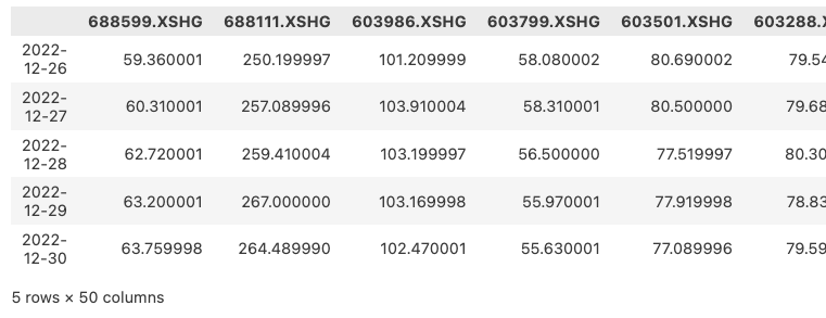
start = datetime.date(2022, 1, 1) end = datetime.date(2023, 1, 1) prices = await get_prices(SH50_CODE_LIST, start, end) prices.tail()

123456789101112131415161718192021
We will obtain the following result:

![](https://cdn.jsdelivr.net/gh/zillionare/images@main/images/2023/12/mpt-5-price-df.png)

We plot the price trends of each asset as shown below:

![](https://cdn.jsdelivr.net/gh/zillionare/images@main/images/2023/12/mpt-equity-wave.png)

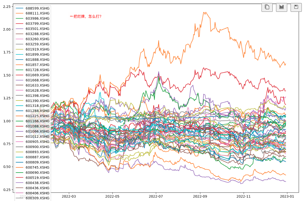
The trick in the above code is likely on line 24, where multiple dataframes are concatenated row-wise to form a wide table. This format was also used when performing factor analysis with Pyfolio.

### Calculating Covariance

In previous examples, we calculated covariance manually. In practice, we can use the `cov` function of pandas DataFrames. In PyPortfolioOpt, we can also use its provided `sample_cov` method:

```python
from pypfopt import risk_models
from pypfopt import plotting

sample_cov = risk_models.sample_cov(prices, frequency=252)
sample_cov.head()

The result is as follows:

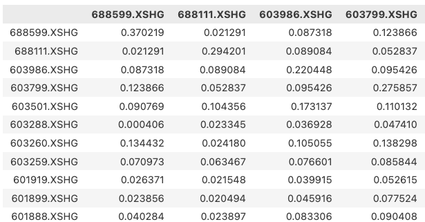
The difference is that if we use PyPortfolioOpt’s sample_cov method, we do not need to calculate returns or handle invalid values separately. This single step accomplishes the following:

123prices = ... # pd.DataFrame, price of each instrument
returns = prices.pct_change().dropna(how='any')
cov = returns.cov()

We use the following command to visualize this matrix:

1plotting.plot_covariance(sample_cov, plot_correlation=True)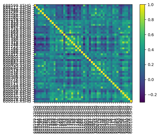

Solving for the Optimal Portfolio

We solve for the optimal portfolio based on conditions such as maximum return and lowest volatility:

123456789101112131415161718from pypfopt import EfficientFrontier
from pypfopt import risk_models
from pypfopt.expected_returns import mean_historical_return

mu = mean_historical_return(prices)
S = risk_models.sample_cov(prices)

ef = EfficientFrontier(mu, S, weight_bounds=(0, 1))

# 求解出最小波动率时的权重
w = ef.min_volatility()

# 输出最小波动率时的年化收益、波动率和sharpe
ef.portfolio_performance(verbose=True)
df_w = pd.DataFrame(np.array([item for item in w.items()], dtype=[("code", "O"), ("w", "f4")]))

# 显示权重
df_w.head()

The usage is straightforward. First, we calculate the mean return and construct the risk model. Since we are using a mean-variance model, we return this model via sample_cov.

Then, on line 8, we instantiate the Efficient Frontier object. It takes three parameters: mean return, risk model, and weight constraints.

On line 11, we optimize for minimum volatility. The result is the weight vector (represented as an OrderedDict). We can manually calculate the corresponding portfolio annualized return and Sharpe ratio based on this vector, or we can use the built-in portfolio_performance method in pypfopt, as shown on line 14 of the code.

Finally, we convert the weight vector into a DataFrame for display, purely for aesthetic reasons.

Thus, we have obtained the expected return, asset allocation (i.e., weights), and their Sharpe ratios and other metrics when volatility is minimized.

Visualization and the Efficient Frontier

The method we just used generated only a single optimal portfolio. However, often we may wish to obtain the entire efficient frontier.

1234567891011121314151617181920212223fig, ax = plt.subplots()
ef = EfficientFrontier(mu, S, weight_bounds=(0, 1))
ef_max_sharpe = ef.deepcopy()
plotting.plot_efficient_frontier(ef, ax=ax, show_assets=False)

# Find the tangency portfolio
ef_max_sharpe.max_sharpe()
ret_tangent, std_tangent, _ = ef_max_sharpe.portfolio_performance()
ax.scatter(std_tangent, ret_tangent, marker="*", s=100, c="r", label="Max Sharpe")

# Generate random portfolios
n_samples = 10000
w = np.random.dirichlet(np.ones(ef.n_assets), n_samples)
rets = w.dot(ef.expected_returns)
stds = np.sqrt(np.diag(w @ ef.cov_matrix @ w.T))
sharpes = rets / stds
ax.scatter(stds, rets, marker=".", c=sharpes, cmap="viridis_r")

# Output
ax.set_title("Efficient Frontier with random portfolios")
ax.legend()
plt.tight_layout()
plt.show()

Ultimately, we obtain the following figure:

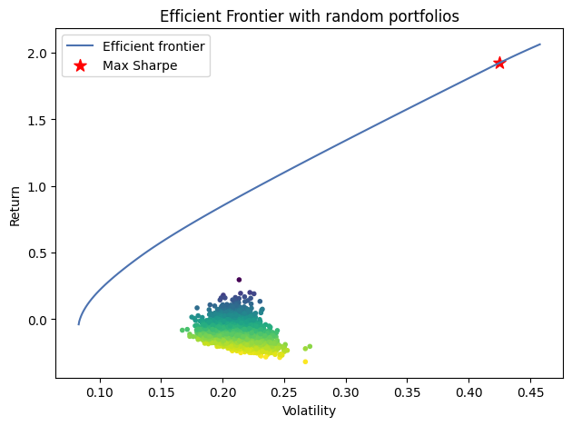
A few points need clarification here:

1. We generated the efficient frontier instance twice. The first was solved using a mean-variance model (i.e., return and volatility), and the second was solved for the optimal Sharpe ratio. Each instance can only be solved once, so we created two instances. Here, we used the deepcopy method, but we could also reinitialize them completely.
2. On line 13, we used the Dirichlet distribution. It is a distribution over the interval (0,1) where the sum of the distribution equals 1. Previously, we achieved this using the following method:

12w = np.random.random(size=50)
w = w/sum(w)

Using the Dirichlet distribution looks more elegant. However, note that the distribution characteristics of the two methods are different.

CAPM and MPT

The previous series covered CAPM. It has intricate connections with MPT. First, when solving for the best Sharpe ratio, we used the term tangency portfolio (see comment on line 6). A tangency portfolio is a portfolio located at the point where the efficient frontier in the risk-return space is tangent to the highest possible Capital Market Line (CML).

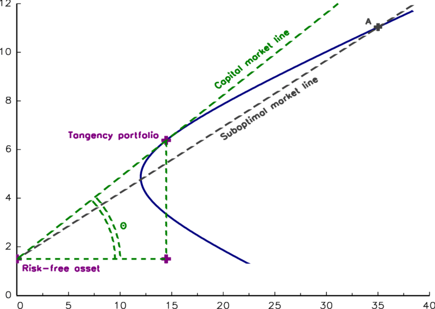
The slope of this tangent line is the Sharpe ratio.

Additionally, in our previous calculations, we used mean historical returns, obtained via mean_historical_return. In reality, mean historical returns have limited reference value because we cannot simply assume history will repeat itself. One possible approach is to calculate the alpha of assets via CAPM and use this as the asset return to calculate the efficient frontier. In this regard, CAPM and MPT theories are organically combined.

PyPortfolioOpt supports this approach. When instantiating the EfficientFrontier object, we can do so as follows:

123456789from pypfopt.expected_returns import capm_return

# 不用历史回报，而改为capm_return

#mu = mean_historical_return(prices)
mu = capm_return(prices)
S = risk_models.sample_cov(prices)

ef = EfficientFrontier(mu, S, weight_bounds=(0, 1))

However, in our example, using CAPM returns might cause an error, indicating that no asset has a positive CAPM return. This is not PyPortfolioOpt’s fault, nor is it our fault.

The market is wrong.

Conclusion

This series on Modern Portfolio Theory concludes here. In this series, besides mastering how to use portfolio theory to manage assets in practice, we have also learned Monte Carlo methods, convex optimization techniques, and how to calculate the Sharpe ratio—important quantitative tools. We also introduced how MPT and CAPM connect. If you are interested in pure theoretical research, you can continue to delve deeper into this area. We have provided some reading materials in the references.

Although modern portfolio theory and other important financial theories are academically successful (winning Nobel Prizes), we must also note that their overly sophisticated theoretical frameworks are often detached from reality. Consequently, they are not highly valued by investment masters who have achieved great success in practice—such as Charlie Munger, who particularly dislikes the Efficient Market Hypothesis and Modern Portfolio Theory.

In Poor Charlie’s Almanack, he wrote:

He also mentioned that one of the world’s greatest economists was a major shareholder of Berkshire Hathaway. Shortly after Buffett took control of Berkshire, he started investing in it. His textbooks always taught students that the stock market is extremely efficient and no one can beat it. Yet, his own money flowed into Berkshire, making him incredibly wealthy.

Nevertheless, learning these theories and mastering the mathematics, tools, and ideas behind them is still very necessary for strengthening our quantitative fundamentals. On the path to learning investing, there is no single theory or system that, once learned, guarantees beating the market. As long as you do not intend to be a scammer in the capital markets, the 10,000-hour rule still applies to you. Starting from the basics, building your own methodology, and gaining insights into the market are the only ways to establish your competitive edge.

This is the principle upheld by the Da Wang Fu Quantitative Trading Course during its compilation. We do not promise to teach you a strategy that can win immediately. Instead, we deconstruct popular quantitative tools and financial theories one by one, reducing them to highly reusable knowledge points, and then reorganize them according to the natural workflow of quantitative trading, thereby enabling students to build a solid quantitative foundation.

References

Yang (ken) Wu: Portfolio Optimization with Python and R PyPortfolioOpt Library PyPortfolioOpt Cookbook Investopedia: Understanding the Capital Market Line and How to Calculate It Princeton University: Mean-Variance Analysis and CAPM Pricing Model CFA Level Test: The CAL and CML